Extending convolution

I propose a new operator which is like convolution so I'll call it covolution for the sake of this discussion:

C = B * M where * is the covolution operator.

The base data B is a set of detail levels of single-bit grid trees of some dimension n, so an example in one dimension:

Additionally you have the mask that applies the change to the base data. This is a mapping from each possible permutation of the local neighbourhood to a new bit value for the centre of the mask. For example for the red 1 in the above diagram, an example local neighbourhood is:

The red position takes into account the three nearby higher level bits, the two neighbouring bits on its level, plus itself, and the two lower level bits below it, then maps this to a new bit value for the red position. This same mapping is applied to every bit in the base data B, resulting in the new covolved data C.

In the example above, there are 8 bits in the neighbourhood, therefore 2^8 permutations to map to 0 or 1. i.e. it is a 256 to 2 mapping which can be stored as simply the set of patterns that result in a 1. Neighbourhoods of any size are allowed, since the operator 'covolves' two arbitrary datas of this structure.

For 2d base data, the higher levels can be thought of as coarser resolution images:

A neighbourhood in 2d may choose the 4 nearest parents, the 9 'Moore' neighbours and the 4 immediate children, requiring a mapping of 2^17 to 2.

You may have noticed that this is similar to Conway's life game, which is a convolution of such a 2d grid with a 3x3 neighbourhood mask. With covolution we can do Conway's life, but the extra detail levels mean that it is continuous spatially, rather than a grid:

This example uses a 3x3 parent neighbourhood only, and the mapping acts to smooth corners and remove some cells that are completely enclosed. It is a covolution applied multiple times to base data with initially only the highest level 4 pixels set to 1. Note that the patterns exist at all scales but don't repeat themselves in a simple way, due to the cellular automata nature of the operation.

Covolution can also apply to real values rather than bits, much as convolution usually is applied to real values. You replace the mapping with simply scaling each neighbour value by the mask value and summing, just as with convolution, much like is done with 'soften' and 'sharpen' filters in image packages.

Further, covolution can apply to any data structure rather than bits or reals, and the mapping can be chosen as any function that maps the neighbourhood to a new value of the data structure.

These are not actually different operations, they all are derivable from the bit version, which is ultimately the most general definition.

Continuous Time Covolution

The covolution operator acts instantaneously. It would be tempting to create an animated set by repeated covolutions: B = B*M, but this is not right, since the 1 dimension of time can't be built from multiple 0 dimensional covolutions. Instead we include scale symmetry to time also:

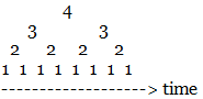
Just like with space, time is also broken into shorter sections for the higher detailed grid levels (like level 1). This leads to an order in which to individually apply the covolution for each level:

1,2,1,3,1,2,1,4,1,2,1,3,1,2,1,....

So a covolution applied in this order is called a covolving system. It is continuous in space and time, and means that the fine details change faster than the larger shapes on the coarser levels, producing true dynamic fractals as seen here:

http://vimeo.com/36816056

Various covolving systems, simply by adjusting the mapping.

The only difficulty is finding interesting mappings. Since there are 2^17 neighbourhood patterns, there are 2^(2^17) possible mappings, which is a large search space.

The trick with finding interesting mappings is to use different constraints to search families of mappings. For example, a simple constraint is to map just the total number of neighbours onto the boolean output. Even with this simple constraint there are still 2^16 possible mappings, here is an interesting bacteria-like result:

http://vimeo.com/36867848

Thoughts on the universe's origin

One of the larger questions in physics or philosophy is where the universe came from. Lawrence Krauss's 'a universe from nothing' video got me thinking about it.

If we think of the universe as 4d space-time then it is just a geometry, unmoving, unchanging. We might ask why this geometry, but a starting question is, why is the time axis so different to the space axes?

Well, relativity tends to deal with how the two relate to each other, but why is there this strong dependency in the time direction?

An answer may be that the universe geometry in 4d is radial around a point, in 2d it might look like so:

The radial lines represent information, since there is a strong correlation along the length of the line, you might say that the direction of the lines (which for a small neighbourhood are roughly parallel) represents the time direction, and the other 3 directions are space directions.

Since the correlation is in this direction, it remains to decide which direction is forwards in time, this is simply the direction to higher entropy.

So I am suggesting that the time dimension is simply the one that happens to be the direction of the lines in this radial 4d shape. It explains why the universe appears to be expanding, is consistent with everywhere being equidistant from the 'big bang', and deals with why there is nothing before the big bang (because that is the centre of the volume), it is approximately the same reason that there is nothing north of the north pole, just a geometry issue with our way of parametising time.

Accelerations or decelerations of the expansion could be explained as changes in the density or roughness of these lines, effectively changing how much time is perceived to pass per unit distance along the line.

OK, so if we accept such an explanation of why we perceive a 3d universe changing through time, then the next question is: why is the universe geometry shaped like that and not some other shape?

We can't ask why there is matter in the universe, because matter is just energy (movement) which is just a correlation of information in the time and space direction. All that exists in this universe is just correlated information.

We can't ask what created this correlated information as we have removed the idea of time and cause and effect, so all we can really ask is: why is the information correlated as it is?

Which can be rephrased as: why are there these constraints on this information?

I can only consider this question speculatively... I am fairly certain that the only sensible answer is that there are ultimately no constraints on the information. In other words, each apparent constraint is an emergent constraint from the action of multiple, smaller level, less constrained information.

This idea can be seen right through physics, from Feynman's path-integral descriptions of particles, to entropic forces which explain elastic forces and probably gravity.

So at the highest resolution there are no constraints and therefore there is nothing that needs further explanation.

i.e. we are living by the high level laws that derive from infinite information acting without rules. Even logic and consistency needn't apply at the lowest levels, it is just that logic and consistency is more persistent, an invariant state or attractor of the mass of possible illogic.

3d numbers

This is the beginnings of an idea about 3d numbers. We have the complex numbers, which are complete, and beyond this we have quaternions and some other constructs, but no 3d numbers. As I'll show, developing a 3d algebra requires moving to multi-valued quantities.

So we have a 3d number a + bi + cj. Addition and subtraction are just element-wise. What about times and divide?

Well, a times b at its core means apply b to a as b is to identity (which is 1 in the reals). Note that this definition works for reals, complex numbers, integers etc.

So like in this diagram, let's say that a is 1+i and b is 1+0.1j. We take the identity to be 1, so b compared to 1 is a relative offset of one vector to another, defined by an angle and a scale, in this case an angle of about 0.1 radians and a scale of about 1.05 or something like that. So that describes how 'b is to identity'.

If we apply this relation onto vector a we have a problem, in what direction do we rotate away from a by this 0.1 radians? We have multiple answers, in fact b could sit anywhere in a circle around a, i.e. b maps out a cone around a, each b having a different phase phi.

At this point we could either say 'well that's no good, a*b must give a single answer' and leave it there. Or, as in this blog, we continue to build the algebra with these multiple results as a feature of the algebra, not as a problem.

So we have a multi-valued algebra where a*b is either a single value when b is a real number, or otherwise is the set of points on the circle of a cone.

So if c = a*b, and c is the circle, then what is c*d? Well for the same reasons it is a thick circle of a cone around a:

This starts to demonstrate that every multiplication makes the result less and less certain.

So, generalising, we can say that a*b is a sort of convolution of b onto a. And, we see that every 3d number is generically described by a probability density function over the whole 3d space.

Also notice that b*a is not the same result, so multiplication is not commutative in this algebra.

In this system we find that addition and subtraction are a convolution of the many-valued quantities, since we're adding all combinations that a and b can be.

Finally, what about divide? Well clearly you can divide in some cases, since it is just the opposite of the multiply. Statistically, we could generate the divide operator as c/b = a for all a and b where c=a*b. However, more work is needed to build a divide algorithm, and it doesn't seem that all numbers can be divided, but that isn't a hard requirement anyway.

So we appear to have a basic many-valued algebra. You can make a similar algebra on the real or complex numbers by allowing dual valued square roots for example, but this 3d algebra has uncertainty at its core. Is there anything more to it than described so far?

Actually yes, the algebra is more complex than it seems. We seem to have some contradictions,

Problem 1: a+a is not the same as a*2 since + is a convolution.

This is where the algebra gets more complicated. You see + is only a convolution if a and b are independent variables, if they aren't then + can act differently.

The way to calculate is to take the phase phi of all the independent variables in the equation as degrees of freedom, then allow each degree of freedom to vary when calculating the result. What we end up with in the general case is a path-integral formula, very similar to the maths of quantum mechanics.

As a result, we get values which are coherent or in phase, e.g. a and b where b=a, values which are out of phase, e.g. a and b where b=-a, and values that are independent, e.g. a and b.

So a*a is not the same as a*b where b is independently the same value as a.

we can draw a single possible phase for a single-value 3d number as a little flag on the end of the arrow, like this:

For a*b where b is independent but with the same value as a, then you get a circle like this, with all possible phases at every point on the circle:

For a*a we instead get the phases rotating with the circle:

Notice that the flags rotate twice around the full circle, since applying the twist phi twice in a*a.

So even though both these pictures are the same probability density function, they will be different if and when they are applied in other operations. For example, if you apply the independent variable d to these circles, you get a thick circle in the a*b case, and something like a thin cardoid in the a*a case.

In fact, we could continue to multiply a by a and get a growing double spiral probably. This roughly defines the power operator, and is much like a spreading wave.

Problem 2: a is not the same as 1*a, since 1*a generates a circle around the vector 1+0i+0j.

We need to distinguish between constants and variables here, we do this by prefixing constants with _. So _1*a = a, but 1*a is a superset of a, constants have phi = 0.

So, getting back to the data structure, a single 3d number is not only a probability density function but also a set of independent degrees of freedom, with a density function for each one. I think.

What is the use of such an algebra? Well it seems to have good links with quantum mechanics. It is interesting that the randomness is a sort of necessary result of extending into 3d.

Living on the hillside

I grew up on the side of a hill. There was always a view ahead of you wherever you were in the garden, and a steep bank behind you. Streams always ran downwards towards the view, ahead of me the future path of the water, and behind me the past.

When asked where the water in the stream came from I might have answered “from further up the stream”, and if questioned further I may have said “well from even further up”. From my knowledge of the garden where I played, and from my friends’ houses it would have been hard to comprehend how the streams could have a beginning and an end… and this isn’t surprising because almost all houses in hilly areas are on the side of the hill, very few indeed are right at the top or right at the bottom, very few places show where a stream actually starts.

As adults we sometimes think of time as flowing like a stream, it always comes from somewhere and goes to somewhere else. And here lies a puzzle for us… what was the first moment in time? And what came before that?

People answer in several ways, some say it’s impossible to have time before the big bang, others say there was just nothing before that, others suggest that there was a big crunch before the big bang, giving way to infinite repeated cycles of universes, so time goes on indefinitely. I would like to explain why I think it is probably none of these.

Just like growing up on a hillside, we are all on a different kind of hill, we are descending from order into chaos. I don’t mean this as dramatically as it sounds, this simply means that things are very very slowly becoming more disordered, it is called the 2nd law of thermodynamics and the chaos is measured as entropy and is slowly increasing.

Unlike what is often quoted of this law, there is not an inevitable march into chaos, but from the high perch of order that we are on in this universe each step in time is highly likely to increase disorder.

In this post I show how the total landscape of possible evolutions of the universe follows a fractal pattern which looks much like a hilly terrain through time, perched on the side of a hill looking downwards to a slowly more disordered future. When we look back towards what we think of is the beginning of the universe we are actually looking up to the top of this hill. As we try and look back deeper into the past the cause and effect of events will become less clear, and a description of why each event happened will be less apparent and more contrived, more and more events will seem to just emerge due to luck from a more chaotic state. This tipping point is the top of the hill.

If we could look back further the events would seem almost magical, things would seem to emerge by change, you might see a chaotic galaxy splitting neatly into two ordered ones, in short it would look like time in reverse. This is because newton/einstein’s physics is time reversible.

So a good way to make sense of this is to distinguish objective time (the horizontal axis below) from subjective time, which always points down the hillside:

Why should subjective time run downhill?

It guarantees that entropy/disorder will increase over time. Otherwise, it may take some clever experiments to explore the relationship between entropy and time, but I will hazard a theory here…

Our perception of time is probably mostly to do with us having memories of the past and being able to store and then re-simulate them in our heads. If you keep memories of up the slope then this has more order and an event uses less information, whereas down the hill events would take more information than our current experience. There is a sense that you can fully know the uphill (past) but are not able to understand downhill (future) as it is more complicated than your current state.

You might even use this idea to come up with a unit of subjective time, the time taken for you to be able to store an event twice in the space that you can currently store an event. This idea lets us answer a second puzzle, how long does the universe last?

If time is perceived in proportion to increase in entropy, then as you near the bottom of the hill, the gradient probably drops off and time will pass faster… i.e. the universe won’t “get boring”… at some point you will hit another upwards hill and you won’t perceive time after that.

Reinterpretation of 2nd law of thermodynamics

It is often quoted that entropy only increases due to the 2nd law of thermodynamics, this isn’t really true in the general case, and the real behaviour is, I think, more interesting and revealing.

The 2nd law is concerned with what happens to certain measurements over time, such as the temperature of an object or the dispersion of a liquid, these measurements are called macroscopic measurements as they measure the collective state, as opposed to ‘microscopic’ measurements which measure the actual exact state of every atom in the object.

Take for example a tin of water-based paint which is white paint in the top half and black in the bottom half. If you leave it for a while it will begin to disperse and eventually the whole tin will reach a grey colour where it will be in equilibrium. The macroscopic measurement is the amount of separation, we could measure it as the vertical distance of the average particle of white paint from half way up the tin:

The 2nd law states that the amount of disorder (called the entropy) increases over time, i.e. the separation level (s) in this tin of paint will go down, which as you can see above, it does. This is because the number of microscopic states (position of the black and white paint particles) for a low amount of separation is far far greater than for a high separation. It is simply far more likely that the set of particles will find their way into the grey state.

To study this more carefully you can grid the paint tin as say 100*100*200 particle positions, and allow each particle to swap positions with one of its neighbours randomly, if you then plot a graph of the dispersion level with time, from any random start point, you actually find that the overall behaviour follows a shape like so:

The usual case for this tin of paint is that its s is 0, it is grey. Occasionally it will raise to a higher level (more ordered) and then come back down again making a little hill. The larger hills are far less frequent than the smaller hills, the resulting shape is a fractal pattern quite different to a single gradient as the 2nd law is often envisaged. This pattern remains pretty much regardless of the actual equations of motion used.

The reason why we usually think of order as always increasing with time is that are examples almost always involve something exceptionally ordered, such as the tin of paint on the left.

The way to think of this on the graph is that, if you searched the graph for a point high enough to represent the separated black and white paint, then you would find it at the top of a very large hill, and as such the projection forwards in time (the slope to the right of the hill top) would have to be decreasing.

Because each larger peak is so much less frequent than smaller peaks, if you find any point of a particular height it is overwhelmingly likely to be the top of a peak as in the above graph. The interesting thing is that this means that, if for instance you search the graph and find a separation level equal to the fairly separated paint 2nd from left in the picture, then if you simulate it backwards in time, the order also decreases. This is perhaps surprising at first, it means that an almost separated tin of paint is more likely to have arrived there ‘by accident’ from a tin of grey paint than to have arrived by being the dispersal of the separated paint on the left tin.

This goes against common thinking, which is that each level of order has arrived from a higher level of order. It is the common thinking that everything has a good reason for its existence, and something or other created it. Because separated paint will inevitably show a dispersion in the middle then a tin with dispersion in the middle must have come from separated paint left for a few hours. This chain of events from order to disorder is common thinking, and it isn’t actually true.

Does this mean that if I go to my garden shed and find a slightly separated tin of paint, that it just got their by accident from an unseparated state? No, because it is still far more likely that the paint arrived in that state by a person putting it there, than by accident.

Does it mean that our history in the universe is actually less ordered than it is now? did we all just appear from some random dust in the last year? Well we have historical records showing order in the past (e.g. photos prior to last year), and even though it is relatively unlikely to have come from a more ordered state, it is much more unlikely to have come from a disordered state and somehow have photos that show it being ordered. In other words, correlating evidence shows us that things have been more ordered in the past, but that doesn’t mean they have to continue to be more ordered in the deeper past.

So my conclusion is that, when we look deeper and deeper into the past, we are looking up to the top of a very big hill like in the graph above. The closer we get to the top, the more difficult the reasoning will become in how events unfolded. That is because they will become less and less causational (downwards slope) and more and more emergent (upwards slope), the other side of this slope will seem like a miracle, as chaos will seem to come together in just the right way, is this miracle actually just time running backwards?

fractal classification continued

In my last post I was investigating the classes of 3d fractal based on symmetric 3x3x3 cube fractals. After looking at the 81 results, it looks like they can be reduced down to 5 class names (cluster, tree, sponge, shell, foam) and 5 class sizes (thin, composite, normal, extended and fat):

The fractals are made of three elements, solid, space and border points. The thin fractals are border points surrounded by space, the fat fractals are border points surrounded by solid.

I realised that the first 3 rows classify the 2d fractals, and 1d fractals are just the clusters, so the table above should generalise most basic fractals. It reminds me of a periodic table actually.

It amazes me how well this table can be used to describe natural scenes:

the set of names above gives a much better description of the scene than for instance trying to describe it out of spheres, polygons etc.

An interesting thing about fractal shapes is that they really define a behaviour as well as a visual shape. For example, it is inevitable that if you put a cluster into a box and try and see if it has a pressure by squeezing the box, then it will have a pressure, just like a gas. Equally a composite tree will brissle in the wind if there is any wind (force) at all, it will behave like a tree, with the large bows moving slowly and the ends shimmering rapidly. A composite sponge will be squeezable and will return to its original shape... why? because any motion given to the sponge's spokes through squeezing it will distribute into seething vibrations (a temperature) of the shape, and through self collision these vibrations will give the fractal an elasticity.

Composite shells are not elastic, since the branching planes prop their neighbours up, so just like their counterpart in nature they are stiff objects, which can encase and protect trees (the shape of most animals) which are flexible.

Thin foam has known and measurable surface area for each bubble and a known and measurable volume of the space in each bubble, as such you cannot change these without it becoming a different value fractal. Therefore surface area and internal volume must be preserved, just like a normal bubble. This means that (assuming the bubbles are not perfect spheres) then due to temperature effects the foam will appear elastic (like a sponge) but preserve volume (unlike a sponge).

The classification table also has an implied 'empty space' fractal right at the top, and 'full solid' right at the bottom. Between these extremes is a curious fractal that doesn't fit into the table, it occurs where all blocks recurse, none are empty, none are solid (#40 on the 3x3x3m cube). The fractal isn't thin and it isn't fat. It contains no solid, therefore it should act like space and objects can pass through it, but it also contains no space, it has a measurable volume of 27m^3 so this volume cannot change without it being a different fractal. Hence it is volume preserving but not stiff. Its inverse is itself, so is half way between solid and space. It seems to me that this fractal should be called 'liquid', as its behaviour seems to match this description quite precisely.

So what I find amazing about these classes of fractals is that, far from being abstract, they really represent the nature of real world objects. A cluster (which is itself a model of gas) has a pressure, sponges are spongey, trees brissle, shells are hard, foam acts like foam. I am not making any concessions here, like pretending solid parts are a bit soft, these 100% precise and accurate mathematical fractals really are spongey, foamy etc, this comes straight from the mathematical definition of each object.

Lastly, under the 'class' category we can give an 'order' to each fractal where the order of a fractal is how many branches it employs each recursion. For example, a binary tree has order 2 and a trinary tree order 3. So higher order fractals are more dense I suppose you could say.

The interesting thing about this is the low orders... a tree order 1 has only one branch each recursion, so can give a spiral or cone. A sponge order 1 has only 1 loop attached to the primary loop each recursion and order 1 foam has only 1 bubble attached to the parent bubble each recursion. These are all valid fractals (even if they don't always give a fractional dimension). They follow all the same rules.

What about an order 0 tree? well this has no branches, it is just a trunk... a euclidean line/cyclinder/blob. An order 0 cluster? the main blob has no children, so is just a blob. For the thin fractals, the order 0 versions of a cluster, tree, sponge, shell, foam are topologically: point, line, circle, plane, sphere.

What this means is that we can classify euclidean shapes with this same system that is used with fractals, they are all one big group. Euclideans are order 0, spirals etc are order 1, fractals are order 2 and above.

I'll finish this post with a fun collage I made of natural fractals, it is a bit of puzzle to discover why each one fits into the box that it is in:

3d fractal types

Even though fractals have been around for half a century, they haven't been really accepted yet as fundamental objects, even though they are generally a better description of natural objects than the euclidean geometry from the ancient greek times.
So, while there is an enormous body of work that categorises shapes such as polyhedrons, it seems fractals haven't really been categorised at all, especially 3d fractals, at least I can't see evidence of this in the public domain.

So today I decided to start categorising. The easiest way to start is to take a 3x3x3 cube (i.e. made of 27 unit cubes) and enumerate the different fractals that you can make with it. For example, if you remove the middle cube and all the face cubes, recursively, then you get the menger sponge.
We simplify the task by reducing the cubes to remove to just the symmetric categories of the middle cube (m), the face cubes (f), the edge cubes (e) and the corner cubes (c), this also has the generalising property that these four categories represent the volume, surface, borders and corners of any polyhedron that might be used in a recursive fractal.

For each category of cube, I choose whether it is outsidethe set (0), recursion applied (1) or inside the set (2). Hence each fractal that I enumerate can be given a trinary code cefm = 1201 (from 0000 to 2222).

Lastly, I want to categorise the *type* of fractals that you can get out of this, not the specific shape. Something more like topology than geometry, but recursive topology.

So here are the results
https://docs.google.com/document/pub?id=1bz0d4RZ9sg_MKJ-3CsIrLxbYUtYOTjKrGLqhsvq3nxE

Most of the names of the types I made up, and I still don't know how to categorise most of these fractals. I think it demonstrates how small our vocabulary is when it comes to even simple fractals like this. Compare it to the euclidean truncated-stellated-hemi-hexahedrons, inflated ellipsoids and non-rational-B-spline-patches etc, where the vocabulary is rich.

I also think there are some fractals in this set that I have never seen before. The branching surfaces are probably the ideal conductors of heat, but I have never seen the shape before. The variation of this #12 which is ridden with holes, and #15 are novel, well to me at least.


People are slowly realising that not only are fractals good approximations of nature but they are also optimal configurations, e.g. a tree shape is the most efficient way to transport water, a fractal coastline is the most optimal way to dissipate the destructive energy of the waves etc. Categorising and creating a vocabulary for 3d fractals seems really useful in this regard.