dimension-aware rasterising

How do you raster geometry? i.e. convert shapes to screen pixels. It might seem like that is a question solved many decades ago but maybe not...

Lets take a simple example of a disk (a filled in circle) which is just black against a white background. To render it we just need to set each pixel to black which is inside the circle right?
Well that is kind of true but not very accurate since we get jagged looking edges. The most accurate rendering would set the blackness of each pixel to the percentage of that pixel which is inside the disk. This gives a slight gradient along the edge which is smoother, it is sometimes called anti-aliasing:

You can see that the left disk looks better than the right disk, it is in fact the best rendering for this piece of geometry. The blackness is proportional to the area of the pixel that is inside the set.

This is in fact how most 2d geometry is rendered, for more complicated shapes it is usually achieved by supersampling, which means testing multiple points inside each pixel (e.g. a 4x4 grid of points) and averaging. This is an approximation of the ideal render since it is an approximation of the area under the pixel that is in the set. It gets closer to perfect as you increase the number of supersamples.

And that's where most rasterisers leave the issue of rastering. But there's a problem, how do you raster a line? You can't calculate the area under a pixel that contains the line because lines don't have area. You could solve the problem by saying that such 'thin' lines are invisible and so you render lines only by giving them a certain width. However this requires choosing a width and it is altering the object to a different shape. We should be entitled to see lines and points and other mathematical objects on our screen, even if they have no area.

In fact you can raster a line on screen, the ideal raster darkens each pixel in proportion to the length of line under that pixel, rather than the area, as seen in the lower line here:

Fine, but what about points? Points neither have area or length. The ideal rasteriser would darken each pixel based on the number of points under the pixel.

And what about rough objects like the Koch curve, this has neither length nor area but somewhere in between, in fact it is a 1.26 dimensional object, but that value depends upon its bend angle.

So rasterising geometry is starting to look very complicated..

Solution

In fact there is a single solution to all these cases, if you know the dimension of the geometry then you measure the 'amount' of geometry under each pixel in units of that dimension. So for the disk you measure the amount under the pixel in pixelWidth^2, for the line you measure the amount in pixelWidth^1, for the point the amount in pixelWidth^0 and for the Koch curve the amount in pixelWidth^1.26 etc. You then darken each pixel in proportion to this 'amount' (The Hausdorff measure). A single method for any dimensional object.

For more general shapes where the dimension isn't necessarily known or uniform we can approximate this ideal rasteriser by using supersampling. For each pixel you count the number of sub-pixels in the set at your maximum resolution (e.g. 4x4 for each pixel) c then you also count the number of sub-pixels containing the set at half that resolution (e.g. 2x2) h. The dimension is then calculated as d = log(c/h)/log(2) and the amount by which you darken the pixel is c/r^d where r is the supersample resolution, e.g. 4 in this example.

Here is the method applied to the Mandelbrot set. Even though the border has dimension 2, the set itself has various geometry of different dimensions within different scale ranges. e.g. there are crooked lines which might have dimension about 1.2 like the Koch curve, and solid areas with dimension 2:

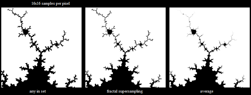
The left image blackens each pixel if any of the 16x16 supersample points are in the set. It has no anti-aliasing and no smoothness even though the curves at the base should be smooth (since I'm only doing 20 Mandelbrot iterations).

The right image is averaging the 16x16 supersample points, it gives smooth curves at the base which is correct, but the line areas at the top fade out and you can't even see the geometry at the very top.

The centre image is using the new method. The base curves are smooth and the line areas at the top are all clearly visible as well as being anti-aliased.

I am using a fractal above as an easy way to get complex geometry, but the technique can work on any black and white image. Possibly it could be extended to colour images too, as a way to retain the important information in an image when sampling to a lower resolution. 

Here's a close up of the above image so you can see the antialiasing:

Here I shade the pixels based on the dimension at that point, viewing part of the Mandelbrot set at 20 and 2000 iterations. You can see the dimension reduces (gets lighter) further up the branch.

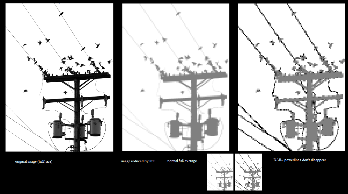
This image shows how you could use dimension-aware rasterising to get useful detail out of downsampled images, in this case showing power lines:

Volcanic surface fractal

This is a short post about a new type of fractal surface.
Simple fractal surfaces are currently rare, which makes finding an example surface for a particular roughness (or fractal dimension) infeasible.
Looking at the simpler case of 2d curves we can quite easily pick a curve for a particular roughness by using a Levy, Koch curve or dragon curve with a chosen bend angle. It would be nice to have an equivalent for a surface.

Here it is, we replace each triangle with 6 smaller triangles of the same shape, with 4 of these forming a diamond based pyramid. Using the pyramid as the base, we parametise the bend angle by choosing the height of the pyramid for unit length base edges. Here are the first three iterations:

If you have a good graphics card and running Chrome then you can see it changing in real-time here:
http://glslsandbox.com/e#4851.17

For pyramid base edge length 1, height h and diamond acute angle a the pyramid and therefore the triangle shape can be fully defined by the equations:

   a = atan(((1+2cos(a)+cos(a)²)/d)^0.5) + atan(((1-2cos(a)+cos(a)²)/d)^0.5)
   d = 4h² + sin(a)²

This shows the fractal with heights from -0.25 up to 1.0.
From 0 up to around 1.75 the Hausdorff dimension increases from 2 up to infinity. The reason the dimension can exceed 3 is that overlapping surfaces 'overfill' the space; mathematically speak, the set is no longer embedded in 3D space.
In fact, as the height increases the fractal 'explodes' out exponentially in size. So it reminds me of a volcano, going from a crater to billowing smoke that covers everything!

When the height is around 0.55 (4th pic from left) the surface is the roughest it can be without intersecting. This has dimension roughly 2.32. The height of 0.5520923 is interesting for another reason, the triangles are all isosceles at this point (angles 1.1697(*2) and 0.8021). It is tempting to think that this might be the same critical point, but not sure.

The Hausdorff dimension D is the solution to the equation:
4A^D + (A/d)^D + (A/c)^D = 1
where A = cd/(d+c) and
c = sqrt(cos^2(a/2) + h^2)
d = sqrt(sin^2(a/2) + h^2)

The model file for the 0.55 surface is available as .obj and .aoi here and here. The surface also discussed briefly here and in this article.

Here's a 2D version, it looks like this for increasing angles 22.5 degrees, 45 degrees, 180*0.29:

Variation:

If you reverse the normals of the sub-triangles in the iteration then you have an effect similar to how the Koch curve differs from the Levy C curve. So you end up with a surface which looks the same whichever side you look at it from:

In this case the largest height before self intersection is about 0.35, as in the picture.

Unlike in the 3d case, the 2d equivalent can go to a larger bend angle before intersecting when its non-V line segment is flipped, here at 45 degrees and the maximum at 60 degrees:

This curve is surprisingly symmetric in its design, and like the Koch curve, you can make a snowflake out of it. 

Mandelbrot physics idea

This is a skeleton of an idea about a possible way to generalise the Mandelbrot set into one that obeys Einstein's field equations and so would represent a 'universe' with gravity and time.

The Mandelbrot set is the constraint Z = Z^2 + C, this can be thought of as its 'law of physics' and it is invariant to any conformal transformation. This is similar to the theory of relativity which defines the laws of physics as invariant to any 4x4 transformation, this is called general covariance. The reason we want general covariance is that it means the laws of physics aren't dependent on any coordinate frame and therefore they are in some sense universal laws. For the same reason the Mandelbrot set is said to be universal, and this is why it appears an infinite number of times in certain other fractals. By the way, it isn't necessary that our laws of physics be universal, but it is massively more likely that we find ourself under universal laws than not.

Equally it is massively more likely that our universe is on the limit set (the invariant set) of its laws than not. All fractals, like the Mandelbrot set are limit sets.

I wonder, if we replaced the Mandelbrot set with M = M*M + C where M and C are 4x4 matrices, then would we have a rule which is invariant to any 4x4 transform? My guess is that we would.
This set of 4x4 matrices could be thought of as the set of energy-stress tensors in Einstein's field equations, or equally the set of tensors representing the curvature of space (since this is proportional to the energy-stress tensor).

Notice that these curvature tensors don't have an associated position in space-time. This is actually what we want because the space-time in general relativity can me many different topologies and we shouldn't expect it to fit inside a single coordinate system.

So we interpret our set of curvatures to be correct and must build our space-time such that it contains only these curvatures. The constraints on how the curvatures should be distributed in space is defined by Einstein's relativity. In particular, there should be no torsion in the space-time, and the space-time should be such that the curvature tensors satisfy the special type of Ricci curvature as defined in Einstein's field equations.

I don't understand exactly how to implement this, but the basic idea is to start at a random curvature tensor in the set and build up the space-time geometry in the neighbourhood based on the subset of neighbouring tensors that you want to use to satisfy the field equations. Each curvature tensor in the set has 16 axes of neighbours, whereas we only need 4 axes of neighbours to generate space-time, so possibly this will help in building the space-time. Additionally, the set should already obey general covariance.
The idea is that you therefore only calculate and see the space-time geometry in your vicinity, no need for a global coordinate system and we naturally get a space-time which is specific to the observer.

You may be thinking that this particular universe will appear to be almost full with matter since every point will have a curvature of some sort. I don't think this is necessarily true, the algorithm to generate a compliant space-time is free to generate as much space and time as it likes, so it could well generate large areas of space between nearby curvature tensors, in order to satisfy the field equations.
Additionally, each curvature tensor can appear many times in many different spots of the generated space-time, since the 16 dimensional set allows the relatively thin 4d space-time to overlap and pass through itself from many different angles.

Summary

So, IF we could write an algorithm to generate compliant space-time to satisfy the set of curvature tensors, then our simple 4x4 Mandelbrot set may be a very interesting 'Einstein universe' to study. Not least because, like the Mandelbrot set, it literally comes from nothing; you start from a zero matrix and simply apply the rule to itself.

This idea also is perhaps a slightly different way of looking at the universe. Space-time is simply the result of interpreting a set of curvatures under a few constraints, it isn't fundamental but an interpretation.

Current understanding of physics

I thought I'd share my current interpretation of how I think relativity and quantum theory work, from a high level. Maybe I'll get time to study them more in future, but here are my current thoughts.

Special relativity

Time is simply an imaginary spatial dimension, so its square value is negative. This is a sufficient premise for describing Minkowski space, time dilation, constant speed of light etc. The rest of the theory is just making mass/electro-magnetic equations etc consistent with this single premise.

Why don't we have galilean (old fashioned) relativity? perhaps because a finite communication speed is more general than a single infinite one, or maybe unbounded communication speed leads to circular dependencies, so cannot be consistent.

General relativity

Think of space-time as a 4d space populated with some 4d vectors (with units of momentum). The distribution of these vectors requires a matrix to define them for each little volume of space-time. Much as a stress tensor defines the stress on an object, this 4x4 matrix defines how dense the vectors are in each direction. If you think of the volume of space-time as a tesseract (4d cube) then the matrix defines the total vector amplitude for a given axis against each cubic side of the tesseract.

This density matrix defines the curve of space-time at that particular point. The curve is the second differential in space of the volume of the space. This curve is represented by a matrix, called the Ricci tensor, Einstein removes a proportion of the trace of this matrix in order to prevent any torsion of space. I believe this is a principle of least work. 

So, if we know our distribution of 4d vectors, we calculate the curvature matrix at each point and we have a space where the second differential is known. An iterative method could take these curvatures on a flat Minkowski space and converge to the warped space-time, which is defined by a matrix at each point (metric tensor). This matrix is 4x4 and looks like a -1,1,1,1 identity in Minkowski space. Bent space-time will deviate from this. 

I think of this as like the 4d vector equivalent of a thermal distribution, where most of the space wants to simply be the mid temperature between its neighbours. That is a scalar example, for a 4d vector you need to work with matrices as this does.

So what are these momentum vectors? they generalise force and mass, if they point in the time direction they are like mass, which moves objects due to gravity, if they point in a spatial direction they are like a pressure and they move objects like a force. Since the curvature matrix is just proportional to the density matrix, a time-pointing vector (a mass) will cause a bend in time, and a space pointing vector (a force) will cause a bend in space. Though it is more of a mixture than this, due to subtracting the trace from the Ricci matrix, I think.

Now that we have a metric for the whole of our space-time, we need to iterate to move the mass distribution, it should shift to only be along the geodesics (locally straight lines in the bent space-time). I'm not so clear how this is best done.

Of course this moves the mass distribution so you have to re-iterate the whole thing continually until it converges to a valid Einstein universe.

Quantum theory

I personally don't see anything weird about quantum theory. It is a set of differential equations (much like most physics theories), the main difference being that it operates on complex numbers rather than the reals. This small difference means that values don't just accumulate, they can also annihilate. The path-integral formulation shows the wave-particle duality in action, a single interaction on a particle is integrated over all space-time and all possible interactions to produce a field (the wave aspect). This is really no different than classical physics formulas using calculus, since differential equations are defining the rules at a single point and requiring they be integrated over space-time to form a field. So no real difference there (apart from the use of complex numbers).

The remaining aspect that people say is different is that the integrated values only define a probability of an effect, rather than an amplitude. This is not actually the case in my opinion. When a simple object like a photon hits a macroscopic object like a recording device, the complex waves decohere and average out to effects that are more classical (amplitudes), the resulting state of the universe contains a spectrum of versions of the same scientist that see the detector light up at different points. Hence it is only natural that any single observer thinks the results are random after repeating the experiment many times. In other words the many-worlds theory seems most sensible and (apart from state-space not occupying a single time-line) the physics of quantum theory is just another set of equations like all the others.

Combining

Since complex numbers are complete, it seems to me that general relativity will need to include complex numbers to work together with quantum theory. This was tried to some degree of success in Twistor Theory, but this theory uses twistors which can't handle arbitrary 4x4 deformations, so can't really get beyond special relativity.
It is true that a 1,-1,-1,-1 metric space is just as valid for general relativity as a -1,1,1,1. This is a rotation by 90 degrees of having i,1,1,1 as the components of time and space. It should follow that any rotation is equally valid, so we have a free parameter in general relativity where quantum objects can be stored... perhaps.

Extending

One problem with these theories is they assume the existence of real numbers, and/or continuums. An improvement would be to define each point in terms of larger and smaller points, so that a continuum emerges in the integration. This is different than normal calculus, but similar to covolution mentioned in a previous post. It also allows certain rules to _not_ produce a continuum but rough (as in fractal) distributions.

alternative relativistic automata

The most general expression of my previous post on relativistic automata can be summarised as follows.
Use any automata rule which updates a cell based on its nearest neighbours, but subject it to this condition:

 For any rule acting on a small volume of space, represented by a 4x5 matrix which defines a position and 4-parellelotope (4d parallelogram) volume, then the same rule must apply to every possible 4x5 matrix and act on the equivalently transformed cell.

The resulting automata has no specific reference frame so is relativistic by design. The direction of the line of time will vary depending on the frame of the observer, and the arrow of time is based on which side has the higher entropy. A simpler way to say this is:

 If the automata turns image A into image B then it would also turn the image of a transformed (sheared, scaled, rotated) image A into an equally transformed image B.

This idea can be partially achieved with regular grid automata as discussed in that post. However regular automata may not allow arbitrary rotations and scale, possible just 90 degree rotations and scale by powers of two.

So a different form of automata may be better in this role.

stochastic automata:

1. place an arbitrary number of 'cells' down randomly anywhere in a 4d space, and set each to either on or off.

2. for each cell, pick n other cells at random to be its neighbours or inputs.

3. pick an arbitrary rule to choose the cell's bit based on its inputs. We can then trial many rules and see what behaviours are common.
4. the automata will then evolve simply by iterating all the cells repeatedly.

Interestingly this basic scheme is all the functionality that is required, the remainder comes down to reinterpreting this data in a way that fits with how we interpret the real world... Here is a first design, lets call it..


Eigenvector Scheme:

In this design the rule is a function of the number of input bits, not the individual bits, so is like Conway's life in that sense:

 a. place each cell in 20 dimensional space, of which 4 dimensions are the usual space-time.
 b. move each cell to the centre of its inputs, in 20d space
 c. the new position of the cell requires re-scaling, stretching and shearing the distribution of inputs so that the 20d cell position is an accurate covariance matrix of its inputs.
 d. repeat for all cells and iterate until convergence.


The expectation is that the cells will order themselves into a network where each cell's neighbours represent nearby points in 20d space. i.e. volumes attach to volumes rather than points attaching to points in normal automata.
We can then decide on some simple rule, such as cell bit = >50% of inputs set. And we can consider the behaviour as reaching some sort of ideal as the number of cells increases and the number of inputs per cell increases to infinity.

The main difficulty with this might be finding the least-work transform to change the inputs into the required covariance distribution. We might want to say that a covariance is only defined by its eigenvectors and values, but that means different points in 20d space have identical meaning. A solution might be to constrain cells to lie only on the eigenvector/value manifold of 20d space.

Reconnect Scheme:
Instead of moving points around in 20d space, we could alternatively try re-connecting the graph into one that satisfies the rule at the top of this post.

 a. place each cell in a 20 dimensional space, representing the 4x5 skew shape for the cell connections.
 b. for each cell, find the closest neighbours in the 16 'covariance' dimensions, 2 for each dimension.
 c. move the cell to the centre of these neighbours.
 d. for each cell, find the closest along-axis inputs for its required matrix shape, 2 for each dimension, so the eight unique inputs closest to where they should be.
 e. move the cell to the centre of this shape and move the inputs to exactly match that required.

The rule then acts on 40 individual inputs per cell, allowing more rules than the above scheme.
Unlike the previous scheme, this one doesn't have ambiguity with several covariances having the same meaning because we are dealing directly with a grid-like scheme. The problem is that reconnecting inputs creates a non-smooth iteration which could jump around and potentially never converge.

Grid-annealing Scheme:

 a. at equidistant points in 16 dimensional space, place and connect points in a grid which is shaped by the covariance matrix at that 16d point. This results in a 20d set of cells with 8 inputs each.
 b. for each cell, find the 32 unique nearest neighbours in 20d and make then inputs
 c. the 40 inputs all have a preferred 4d position, iterate shifting the cell positions to descend towards an approximation.

This scheme is simple to implement and will definitely converge. But it may not be ideal as the grid-like connections probably don't make it optimal.
It seems sensible that not only should the 4d spacing be affected by the covariance, but also the 16d spacing. So that matrix variations are closer together on small grids. But this gets harder to picture when we consider the stretched and rotated spacing for a general 4x4 matrix.

Convolution automata:

Although the idea of relativistic automata is simply stated (top of post), it is hard to find an algorithm that will implement it. Grid-based methods seem too constrained, you can't rotate by a random angle and get the same results for example. Stochastic methods may get around this by breaking the rigid grid symmetry, but there is no clear best approach as yet.
More-over, the idea of expanding the Minkowski symmetries (rotation, boost, translation, scale) to full 4x5 transforms is speculative. It relies on certain of those matrices naturally being somehow not seen by the user.

A different approach is to expand convolution, so move from bit fields to real numbers.
Convolutions usually convolve over space, but here we make them convolve over volume too:

1. take a 4d grid of real values, and a convolution kernel, for example a 3x3x3x3 grid of real coefficients.
2. convolve the grid (i.e. apply the filter to every position on the grid), this could be considered as a convolve for a kernel scale matrix of diagonal (1,1,1,1).
3. repeat the convolve for a different scale matrix of (0,0,0,2), this is equivalent to scaling the kernel by two in the 4th dimension. Add this new convolve on top of the previous.
4. repeat again for diagonal matrix (0,0,0,3) and again up to (0,0,0,n)
5. in fact repeat this for every integer 4x4 matrix (not just diagonal matrices), each one equates to a transform of the original kernel.

And there we have it, a matrix-independent automata.
One problem is that the size of the result will grow as the convolution range increases. So it might need a reducing scale factor with size... so that it appears the same at all possible scales and transforms. You could weight each convolution based on the 4-volume of the transform, or perhaps more efficiently, you could use non-integer transforms, varying the gap between each transform based on its volume, such that the total effect at each volume is probably proportional to the 4th root of that volume.
An unanswered question is whether higher resolution (small gaps between transforms) converges to a solution or whether it somehow averages out to just give a blurry mess.

Relativistic Folding Fractals

Although this may not class as an automata, a simpler scheme to generate 4d shapes with some transform symmetry is to extend the idea of Kaleidoscopic Iterated Function Systems. It works like so:

 1. for each point in 4d space-time, apply some transform to the point, composed of:

    a. rotations

    b. translations

    c. scale (enlargement)

    d. boosts

    e. folds

 2. repeat up to n times (larger n is more accurate)

 3. draw the points that stay within a certain 4d Minkowski distance, which is defined as sqrt(x^2 + y^2 + z^2 - t^2)

The folds can be a reflection in just the x axis or the t axis. The boosts, translations and rotations allow the equivalent of any possible fold. Equivalently you could define fold operations about any 4d axis and 4d point.

Here I have a simple implementation: http://tglad.powweb.com/relativisticFractals.html

This is the bare minimum relativistic version, we could also try expanding the fractal to include any 4x5 transform (plus folds), this fractal makes it easy to try out different combinations.

Relativistic automata continued

Previously I covered some ideas about fractal automata and extending it to a kind of relativistic version. I'll summarise this then describe some thoughts on extending the system to be more relativistic.

translation

Starting with simple cellular automata, like conway's game of life, we generalise it by saying that the function acting on each cell (which chooses whether to turn the cell on or off) can be any function of n nearest neighbours. Typically we pick some small set, like the 9 neighbours in a 2d grid (including the centre one). Giving 2^n possible neighbour patterns and 2^2^n possible functions. The choice of function isn't too important here, what is interesting is the type of results you get by searching through the set of functions as applied to initially random data.

scale

We can expand this system to fractal cellular automata by using a grid tree rather than a single grid, the nearest neighbours for each cell include those on the parent and child grids as shown here:

The coloured cells being example nearest neighbours of the red cell. Typically you watch the highest detail grid evolve. This system effectively gives you a continuous euclidean space, which is more physically real than a discrete grid.

non-uniform scale

These grids can be 3d too, or even 4d. But to deal with time properly we need to use a Minkowski 4d space rather than a euclidean grid. It can be approximated by making the time axis the long diagonal of the 4d grid and allowing non-uniform scales, i.e. cuboid grids. So just as scale becomes like an extra degree of freedom in fractal automata, we let scale in x, y and z separately become three extra degrees of freedom. As discussed in my previous post. The non-uniform scale allows the same rules to apply at different velocities, which are represented by the different non-uniform scales.

At this point there are actually two ways that you can work with time here, you can make the cellular automata only depend on cells that are further back in time, which means that the automata spreads forwards along the time direction:

Or you can keep the cells dependent on all the neighbours (both forwards and backwards in the time direction). This means that a whole span of time evolves as you iterate the automata. This second method has three possible outcomes:
1. The evolving automata converges on a fixed result. This can then be 'played' as a single time line.
2. The automata ends up in a cycle, so no single time line exists, but you could consider each result as being parallel time lines.
3. The automata doesn't settle into a cycle (so is a strange attractor). This has some similarities with the many-universe interpretation of quantum theory, since there are infinite time lines, describable by a probability density function. So any of the time lines is a valid result, after it has converged.

symmetric sheer

The next step is to allow a diagonal stretch of the grid. This corresponds to information which changes more or less slowly with time:

This feature is part of general relativity, time is more dense close to high mass objects. This change in the 'speed of the physics' is what causes objects to fall under gravity. It hasn't been tested, but the idea is that moving points will deflect into the higher density areas, causing something vaguely like gravitation.
This extension has some problems which require a further addition to solve; the stretched grids have a different apparent maximum velocity, inconsistent with the real world.

I have headed the sections in this post to show the different symmetric transforms that each algorithm adds to the system. Continuing this theme and generalising, a square cell can be transformed by any transformation matrix. So there are a few remaining degrees of freedom that can be added as extra symmetries:

rotation

If the path of massive objects is allowed to rotate with time (as opposed to a boost, which is the non-uniform scale above) then the object will be able to attain just as high speed as a light object, which is physically real. However it doesn't appear to obey special relativity since the rotation could make any object go faster than some maximum (light) speed. 

I think the way this is avoided is that the frame that we visualise is the square (not uniformly scaled) frame, and the frame of heavier objects is 'ghosted' onto this square frame, just as low resolution objects 'ghost' onto the high resolution mesh that we view. The ghosting process prevents the object going faster than light since it can't ghost beyond this speed.

This is again a bit speculative, but it seems that the movement of a high mass (stretched) grid can only change direction over a longer period of time, in other words its acceleration should be less in general, and would be symmetric to higher acceleration in a lower mass object.

non-symmetric sheer

The final degrees of freedom are non-symmetric sheering of the cell. This relates to symmetric sheer much as pressure relates to mass or energy in general relativity I think. So for a 4d space-time, the general transform would be a 4x5 matrix, giving 20 dimensions to the cellular automata.

dealing with scale problems

The problem with using symmetric scale for mass is that the stretch only jumps by some fixed factor, like two.

Similarly, the problem with using rotation with time to give a mass a velocity is that grid-based cellular automata can only rotate by 90 degrees. 

The solution to such problems might be to treat the scales (which are the rows of the 4x4 matrix) the same way as position is treated (the 5th row), i.e. use the overall scale to allow each row to be continuous. 

I'm not sure how well this idea works, so this problem leads to a completely different formulation that I will discuss in the next post.

Summary

Space-time is usually thought of as a 4d continuum of points, something which could be naively modelled as a 4d grid cellular automata. 

Instead, if we think of space-time as built of 4d volumes then the description of such volumes which is independent of any reference frame is one which is symmetric to any 4x5 transform. This is quite similar to the principles of special and general relativity. Such a 20 dimensional automata could potentially have the following extra realisms over basic cellular automata:

1. It is continuous

2. parts can have velocity

3. nothing goes faster than light, time dilation etc of special relativity
4. many-world timelines, consistent with some quantum effects

5. mass affecting how fast something accelerates
6. gravitational wells (general relativity)

7. attraction based on pressure (also part of general relativity)

Quaternions aren't rotations

Recently I discussed the difference between unit intervals and integers. Unit intervals are kind of the complement or the opposite of integers, they represent the whole space between each integer, and you could say that they represent the full transition between each consecutive integer.

This is relevant because I was recently reading about the spin group Spin(n) and the special orthogonal group SO(n). The special orthogonal group can be thought of as an n dimensional rotation matrix and the spin groups are spinors which kind of represent rotations as well, but have the confusing feature that you need to travel 720 degrees to return to the same spot. The 3d spinor is the same as the quaternion.

Spinors are confusing, as illustrated by Michael Atiya (from the Wikipedia article on spinors):
"No one fully understands spinors. Their algebra is formally understood but their general significance is mysterious. In some sense they describe the “square root” of geometry and, just as understanding the square root of -1 took centuries, the same might be true of spinors."

It dawned on me that spinors are to the rotation matrices what intervals are to the integers. Spinors are the full set of configurations between two rotation matrices. So they do not represent attitudes (orientations) themselves.

Looking at the 3d example, the attitude of an object is its 3x3 rotation matrix. If you attach that object by many elastic strings to a reference frame (like to the walls of the room that it is in) then the 3d spinor (which is a quaternion) represents the configuration of the strings (which do only repeat after a rotation of 720 degrees of the object). 
So in this example the rotation matrices are the object and the room, and the quaternion is the strings. It is a full path (or interval) between two rotations, which is quite different to a relative rotation matrix.

To rotate a vector v by a spinnor s, you do: s' * v * s. Same for rotating a rotation matrix by s.
The reason for the double operation (which also explains the double cover) is easier to see if you convert back to the integer and interval analogy:


Integers are just points, which really convey no size. In order to add 1 to an integer, first you must append a unit interval from the integer (think of laying down a metre rule from that point), then you must append the point to the other end of the unit interval, so you are doing the first operation kind of in reverse. 
In fact, for any vector you can move to a different vector position by laying down a straight line (an interval) from the first point, then placing the new vector at the other end of the line.
This two-stage symmetric operation can be defined as s' * v * s.


So in fact, basic arithmetic and vector operations can actually be done using these two complementary objects (the point and the interval), we just don't usually think of it that way as we have a simpler system of adding only vectors. But this two object system is exactly what is required for operations acting on orientations.