8 types of shape

A random thought from the other day is that shapes can be categorised by the presence or not of faces, edges and corners. That's a 3D table so I'll fill it in as two 2x2 tables:

faces:

	Edges	No edges
Corners
No corners

no faces:

	Edges	No edges
Corners
No corners		.

For the object with no faces but edges and corners, you can see the corners as protrusions on the top side, and the edges when viewed on the bottom side.

The spikey object (bottom left) with only appears to have corners because I have cropped it to finite size, but the basic structure is unbounded and all those corners connect to another to make continued curved edges.

The object with no faces, corners or edges is probably just a point, or just nothing.

Many-valued Polynomials

Multi-valued algebra promises to help with multi-valued problems such as: if x^2=1 and y = 2x then what is x+y? They aren't super popular as it is hard to make them into them into something consistent like a proper mathematical field. But never mind hey.

Let's define a multi-valued algebra as one where each element is a closed set of complex numbers, let's call the set of such closed sets M. Equality is set equality, summation is the Minkowski sum, and subtraction is the inverse of the Minkowski sum (which doesn't always have a solution).

Let's use capital letters for members of the multi-valued algebra, and lower case letters for single complex numbers.

In this system a 'complex linear multi-valued polynomial' means the complex-valued function:

y = aX + b

Which only occurs when X has a single element, so not very interesting.

a 'complex quadratic multi-valued polynomial' is:  

y = aX^2 + bX + c

which for the specific case a=1, b=-1, c=0, can be written as:

X = X^2 + y

which is reminiscent of the Julia set iteration for each y. 

Indeed the value of X is indeed a Julia set of that complex number, as it is the largest closed set that satisfies the equation. It also remains a Julia set when a,b,c are different values, just with a Euclidean transform applied.

So the function M->C is defined for Julia sets, and each Julia set is the preimage of its corresponding parameter y.

If we 'expand out' the domain into its individual complex elements then the function becomes a many-to-many map m(z): C->C, and m(0) is the Mandelbrot set. So the Mandelbrot set is the image of the number zero under this mapping. More generally m(x) are the generalised Mandelbrot sets that start at point x.  

Above: m(0.3i) and m(0.3-0.3i), these are variants of the Mandelbrot set.

We could approximate this idea by saying that the quadratic polynomial's "multivalue-range" is the generalised Mandelbrot sets, and its domain is the Julia sets.

While we have done a lot of hand waving here, the interesting result is that Julia sets and Mandelbrot sets are fundamental elements of multi-valued quadratics. Fixed y cross section is a Julia set and the fixed z cross section is a Mandelbrot set. 

I haven't explored higher order polynomials, but it seems probably that these produce higher order Julia sets and the higher order 'multibrots', and perhaps linear combinations of these at each order.

This is a nice idea as it suggests that Julia and Mandelbrot/Multibrot sets are the fundamental elements of this multi-valued algebra. If we make the leap that standard algebra is missing something in its inability to answer questions such as the initial one, then we may even consider Julia and Multibrot sets to be fundamental quantities more widely in algebra.

To add to this, the Multibrot sets are universal objects, which loosely means that you will find them in bifurcating mappings. 

The mapping m() can also be seen as a four dimensional shape. In this shape the Julia sets are the horizontal cross-sections, and the generalised Mandelbrot sets are the orthogonal cross-sections. It would be interesting to see what diagonal cross-sections look like.

Disk Cluster

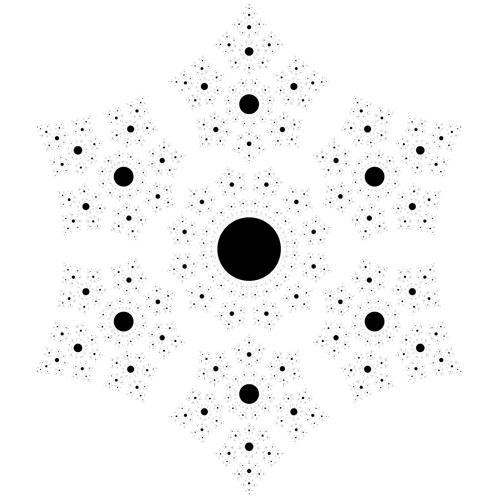
 Here is a nice example of a cluster.

A cluster is a recursive set of separated solids. It isn't too hard to make an example of one using squares, but harder with disks. In this case I wanted an example with no smooth (differentiable) surface, just as the Koch curve and other fractals have no smooth parts to them. 

It is a little hard to see in the image above, but you couldn't 'land' on any of these disks as there are increasingly small disks towards the surface. 

My first attempt was quite interesting because it contains a Koch snowflake within it (can you see it?):

But the relative structure between clusters changes as you go inwards towards the centre, it also means that the outer shape almost definitely self-connects so isn't a cluster at all. 

The top image however applies Mobius transformations to each cluster so that the gap between clusters remains similar all the way down. Everywhere is disconnected, and it also gives it nice point corners.

A less spikey cluster can be achieved by rotating the shape each iteration:

Mean Brownian Paths

Brownian motion is a pure random process and produces paths that are each and very squiggly. In fact so squiggly that their fractal dimension is 2. 

But what about the shape of the path on average?

For any particular section of a random (Brownian) path, we can perform a least squares alignment of every such path and draw the mean path shape:

It is straight because there are as many trajectories that bend anticlockwise as those that bend clockwise. But we are interested in paths rather than trajectories, and the time direction doesn't matter with paths. So here we find the closest Euclidean alignments for either time direction:

It is (I very much suspect) a circular arc. The angle of rotation of this arc would be an interesting constant to discover, it seems to be 1 radian, but that is a rough guess. The bulge is about 0.152 of the arc length, which is interesting because that is exceedingly close to the proposed solution to Moser's worm problem, which is an arc displaced 0.1528 at the centre (An Improved Upper Bound for Leo Moser’s Worm Problem). Moser's worm problem is to find the minimum area shape to accomodate unit length curves, the above curve is the mean unit length curve, because Brownian motion over a unit length is statistically the set of all unit length curves with no bias. So it is interesting that the minimal area shape is potentially a reflected pair of these mean curves:

potential minimum area solution to Moser's worm problem. Bounded by two similar arcs to the mean Brownian path.

The mean curve has bilateral symmetry because we don't allow mirroring in our equivalence class of path shapes. If we do allow mirroring we get:

The two images were for a different number of vertices and different random values, to show that the shape is consistent. This is an average path if you allow flipping, so its mirror image is the other equivalent average path.

You might be wondering what would happen if you don't allow time symmetry but you do allow mirror symmetry. The result appears to be exactly the same as just time symmetry and no mirror symmetry. This makes sense to me. 

Brownian motion in 2D inevitably crosses over itself to form a loop. If we look at just these loops when we get a similar set of results. If time symmetry is disabled then the average circuit is a straight line back-and-forth motion:

If it is enabled then we get a bilaterally symmetric shape:

Here are the points (separate run):

and if we allow mirroring in our equivalence class then we get this funny shape:

and its reflection  (separate run):

We generate these loops because each axis in 2D is performing Brownian motion, which we can model at large scale as a normally distributed offset between each point in turn. In order to get a loop we need each axis to return to the original value, which is called a Brownian bridge. Rather than running a million times until it happens to return to the same value, we simply subtract the linear function from start to finish, which is proven to be equivalent. 

So there we go. Since Brownian motion is a purely random process, these shapes are sure quite relevant as the bulk shape traced by random paths and random loops. We might even think of them as archetypal paths and loops, as they don't seem to contain any prior information, just randomness.

Since there is no prior information in the formulation, the shapes are pretty much definied by the equivalence class used. If you know what your symmetries are when declaring two shapes to be the same, then this dictates what the shape will look like; the result is a function of your interpretation of what a shape is.  

Between a tetrahedron and a sphere

What's in between a tetrahedron and a sphere? You could smooth the tetrahedron partially but this no longer has any flat sides, or you could go to higher solids like an octahedron then an icosahedron, but these still have sharp edges, unlike a sphere.

A polyhedron has C0 continuity and a sphere has Cinfinity continuity. It makes sense that an intermediate could have C1 continuity, which is what this shape has:

We start with a tetrahedron:

then slice off the corners and the edges:

and repeat:

the limit as the iterations goes up is:

I am just showing the edges, but this is a convex solid with flat surfaces in all the circles. In this one the corners are cut off so the slices touch, and the edges cut off one third of the way along the sliced edges. The result has octahedral symmetry, with 8 largest circle faces. 

It is C1 continuous because its face angles (the first derivative) follow a devil's staircase function across an edge, this is a continuous function. 

Here's the solid object:

and here's the same thing but starting with a cube:

Here is the Octahedral rendered with transparency and refraction:

Mean Lumps

So what does a mean shape look like overall? I'm talking about any sort of blob-like shape. A rock, a piece of dough, a pebble, a chunk of ice in saturn's ring. 

This parameter space is pretty hard to pin down, and each of the above have different processes that form them. But one common thing is that they are fairly smooth, and they have a continuous, simple surface. We aren't talking about sea urchins or sponges or tree shapes. 

Regardless of the exact parameter space, the average shape is constrained by the equivalence class, and it is due to this that we can get a rough shape, without knowing the actual probability density of the parameter space. 

In this post I make an attempt at an average shape using an octahedron with randomly selected radial distances of the six vertices, using a random distribution of 'energies' (the square of the distance) as used in previous posts. In fact we already have the result, it is from the dice numbers in the mean textures post. The dice values for the sides 1,2,3,4,5,6 are: 3.35, 2.57, 2.86, 2.86, 4.58, 5.98, which translating to radial distances gives this shape:

The left side is the octahedron from three angles, and the right is a smoothed version to give an idea of the blob shape. As you can see, it has bilateral symmetry, but is elongated and somewhat egg-shaped in the two other axes.

We can do the same thing with icosahedra. The result is:

vertices: x: 1,-1, 0, ϕ, ϕ, 0,-ϕ, 0, 1, 0,-ϕ,-1
               y: 0, 0, ϕ, 1,-1,-ϕ, 1, ϕ, 0,-ϕ,-1, 0
               z: ϕ, ϕ, 1, 0, 0, 1, 0,-1,-ϕ,-1, 0,-ϕ        (ϕ is the golden ratio)

lengths: 1.03,0.91,0.91,0.92,0.92,0.90,0.93,1.65,0.93,0.93,0.93,1.04 

The result is a bit different, but the main features are similar to the octahedron case: It has bilateral symmetry on one axis, and an egg-shaped elongation on the two other axes, the proportions of these two elongations are similar with the octahedral case, the main difference being that the icosahedral blob is fatter (bottom row).

Nevertheless, these two blobs are quite similar looking, and remind me of an almond a bit.

Mean particles

The results of the previous post on mean points shows that average sets of points tend to not be next to each other. If we introduce time into the system, then this can be seen as a repulsion of the points. So let's try this out. 

Looking at just points in a 1+1D world, where the spatial dimension is in a circle. We can evolve a set of points as follows:

1. Pick any set of starting points, these are also the current mean point set.
   
2. Create a large population of sets, each set is equal to this starting set. 
3. For each time step, add a random offset to each point set, and rotate it around the circle to be as close as possible to the mean set. Accumulate the deltas (relative angle of these rotated points to the mean points).
4. add the total delta onto the mean point set. (i.e. generate a new mean set)
5. go to 3.

 The results are shown with time going from bottom to top, with starting positions 1,1.1,7,8  (angles out of 10 ticks around the circle):

Notice that points appear to repel each other, and the two points closest to each other repel the quickest.

The size of the random offset applied at each time frame affects how fast the particles communicate and 'see each other', with no repelling until the random dispersion of each point starts to interfere with its neighbour.

Since we use a large population of random sets, it basically represents a uniform dispersion of the sets over time, with a chosen dispersion rate. The dispersion rate does not have any effect other than changing the time scale on the resulting trajectories. So the results are effectively parameter-free. They are simply the mean trajectories of a set of n points, given the circle's rotational symmetry, and a maximum communication speed. As such, the trajectories are otherwise entirely defined by the initial position of the points.

The behaviour isn't particularly interesting though, but we can make it more so by going from first order to second order dynamics. This is done by adding the change in the mean points on to all the candidates at each time step, reflecting the nature of particles to maintain their velocity. The result has a little more oscillation:

This is basically degeneracy pressure in action, just without complex numbers. However, there is an additional behaviour in this system: unlike degeneracy pressure in absolute coordinates, which converges (if it loses energy over time) to equidistant points, with circular symmetry included the points stabilise to the non-uniform dispersal seen in the previous post. At least it would if the communication distance was wide enough.

This makes it a system that has repulsion and a sort of attraction (as the converged set of points cluster on one side of the circle). This is not visible on the above graph due to the communication distance being lower, but it would be interesting to investigate this behaviour further.  

I expect the 2D version (on a sphere) to show even more unusual behaviour, it could well display orbiting behaviour around the lowest energy point locations (seen in the previous post).

Also note that the set of particles conserves momentum. At least, it appears to.