Mean Transformations

A while back I looked at mean polyhedrons and said that the mean cuboid should have sides of length (2,5,11) or (1,2.5,5.5).

A different way to estimate a shape's principle dimensions is to represent it by a random transformation of a sphere by a transformation matrix M. The eigenvalues of that transformation then give the principle dimensions of the resulting ellipsoid. This can be done in any number of dimensions and just requires a decision on what a random nxn matrix should look like. 

If seems to me that what I should really do is treat it as a n^2 length vector with equal likelihood of pointing in any direction. This is easily achieved by sampling each vector element from a N(0,1) normal distribution, then normalising the vector.

I then order the eigenvalues by their absolute value and average them over 300,000 randomly sampled vectors representing the matrix M. The resulting shape dimensions for each number of dimensions is:

1: 1

2: 1, 2.34, 

3: 1, 2.70, 4.41 

4: 1, 2.393, 4.23, 6.04

5: 1, 2.532, 4.096, 6.130, 8.16

6: 1, 2.412, 4.06, 5.67, 7.77, 9.90,

7: 1, 2.486, 4.02, 5.774, 7.475, 9.705, 12.0

8: 1, 2.417, 4.00, 5.557, 7.35, 9.084, 11.371, 13.731

9: 1, 2.464, 3.99, 5.65, 7.27, 9.14, 10.95, 13.33, 15.82

10:1, 2.420, 3.98, 5.524, 7.214, 8.856, 10.756, 12.61, 15.04, 17.61

A few interesting things to note:

1. The pattern is not simple, the second extent for example oscillates, perhaps converging towards 2.44 somewhere.

2. The third extent however just decreases, converging towards 3.95 perhaps

3. The fourth extent also oscillates, the fifth decreases and the sixth oscillates... do only the even extents oscillate?

4. They all seem to converge, suggesting that there is a value for the infinite dimensional shape. 

5. The shape is quite different to the previous mean ellipsoid for the 3D case. That one was more cylindrical, this one is more planar.

6. For each dimension the sequence grows superlinearly. Is there a pattern?

If we look at the difference between consecutive extents in the 10D case:

1.42096, 1.55935, 1.54375, 1.68965, 1.64261, 1.89974, 1.85389, 2.43466, 2.56585

You'll notice that this is also not smooth, it oscillates, though this time while growing. The same is true for all cases < 10D too. So none of the extents seem to follow a simple pattern.

Update: this topic seems to be exactly the subject of Random Matrix Theory, and the above eigenvalues should tend to a semicircle distribution if I'm understanding it right. The oscillations appear in the link for finite values of n (probably causing the oscillation with respect to n too):

 The simple takeaway is that as n tends to infinity, the distribution of Eigenvalues will tend to a quarter circle (or a semicircle if we allow negative eigenvalues). This semicircle histogram is because the eigenvalues (in the complex matrix case) tend to a uniform unit disk distribution.

Saturated and desaturated 3D shapes

Saturated

Here are some more examples of saturated shape (see last post), this time 3D. I've used the inversion sets table as a starting point.

These saturated surfaces all have fractal dimension 2, so they are 2D surfaces. However their surface areas are infinite. A measurable area needs to be in m^2 log^n m where n is larger for the lumpier shapes:

These are also saturated surfaces, but this time saturated with spheres rather than lumps or dents:

Neither are fractals and neither have finite surface area. 

These curves all have fractal dimension 1, they are non-fractal (branching) curves, however their total length is infinite. You need to measure their size in m log^n m for some n representing how saturated they are:

(ignore the sphere in the centres of the last one, an artifact of too few iterations)

This set is disparate points, or dust. It's fractal dimension is 0 like its topological dimension, so it is not a fractal. But the number of points is infinite, you need to 'count' the points in log^n m:

So saturated shapes are relatively easy to create in 3D. 

All of these shapes are nowhere differentiable. They are more lumpy than C(1) fractals like the Hevea project shapes which are differentiable and also have finite length/area.

Desaturated

This is a desaturated tree surface fractal. Its fractal dimension is something like 2.5, but the roughness grows at the finer details, such that its area in m^2.5 is zero. 

Here is an equivalent with the cluster-tree fractal:

 

In both cases the desaturated shapes look sharp compared to the rough fractals, and the saturated shapes at the top look blunt.

Here's a desaturated shell-shell:

The equivalent for the void-tree again has most of the geometry at the finer scales:

Saturated and desaturated shapes

Here's an unusual curve:

Its fractal dimension is 1, so it is not a fractal. But its length is infinite. It is constructed like a Koch/Cesaro curve with local dimension D(i) at iteration i given by D(i) = 1+1/i. Where the per-iteration bend angle equals 2asin(exp(-ln(2)/D(i))).

The question is how do you compare the lengths of different subsections of the curve, if they're all infinite? This is reminiscent of the Coastline paradox. 

There are related curves that have local dimension D(i)=1+0.5/i and 1+2/i respectively:

This raises a second question, not only do we not know which is longer, but they clearly change in how lumpy they are. How do we measure that? 

I described them all as lumpy, rather than 'rough' like fractals because the lumps are only at the larger scales. I use the term saturated to describe these curves. Their length has saturated to infinity and it also invokes the idea of a shape saturated and swollen with water like wrinkly fingers in the bath.

This next curve has local dimension D(i) = 1.2618+1/i so it is a fractal, in fact it is the saturated version of the Koch curve. Its fractal length (fractal content or Hausdorff measure) is infinity.

Moreoever if you measured this fractal content for a slightly higher dimension such as 1.2619, it would be zero. So you cannot use fractal content to measure the length of this curve either.

The answer to these problems is that instead of measuring these lengths in metres (or metres^1.2618 for the saturated Koch curve) you measure the in m log^n m (or m^1.2618 log^n m respectively). In general any shape of dimension d that is saturated can be measured in m^d log^n m. Here n is the value that describes their lumpiness. In these examples when the local dimension is D(i) = D + k/i, then n = k ln(2).

The shapes don't have to be curves. This is a particularly pure case of a saturated 0D shape, i.e. a point or finite number of points, where D(i) = 0 + 1/i:

There are infinite points in this saturated shape, but unlike the 2D Cantor set its fractal dimension is still zero, so it is not a fractal. But, you can still compare the size of these shapes (or portions of them) as they can be measured in log^n metres. Here is a twice as saturated set of points (twice n): D(i) = 0 + 2/i:

The point spacing is decreasing as we zoom in. Indeed all of the above examples change their scale and shape as you zoom in. But even though their log-log plots are curved it is still possible for shapes to be scale-symmetric. Take for instance these binary trees:

They both have fractal dimension 1 so are not fractals, just connected lines. If the stem length is 1m then the left image has total length 12 m. But the right shape has infinite length; it is saturated. We can still measure its "length" as 2.88 m log m. This saturated tree occurs when the child branch lengths are exactly half the parent branch length. 

Desaturated shapes

The same thing happens in the other direction. You can take a 2D area and remove the harmonic series. Here the local dimension is D(i) = 2 - 1/i, and 2 - 2/i respectively. They both have area zero, so how do we compare their sizes?

Similarly you can also desaturate a fractal, such as the Koch curve here, using D(i) = 1.2618 - 1/i. Its fractal content is then zero.

The equivalent measurement for these is to measure in m^d / log^n m.

Here's a desaturated solid triangle, with D(i) = 2 - 1/i:

I call these desaturated as their d-volume has all of its size "dried" out of it, like dried ground that has split. In general we can think of these desaturated shapes as dessicated or depleted versions of the original shape.

This next shape is a line using a binary subdivision formula with D(i) = 1 - 1/i:

It looks like a Cantor set but its fractal dimension is 1 and its 1D length is 0. You must measure the size of this desaturated line in m/log^n m.

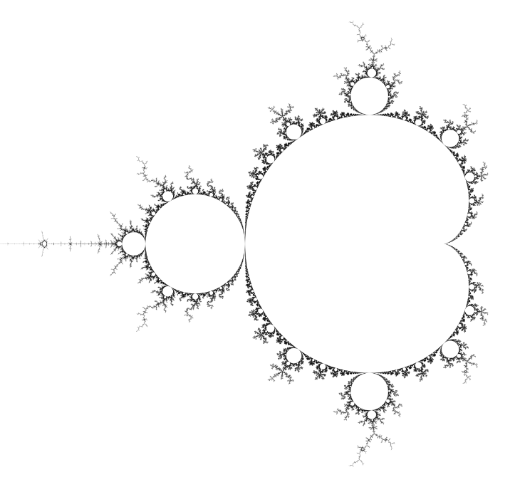
These aren't the only shapes that act this way. If we plot the box counting dimension of the boundary of the Mandelbrot set as a log-log graph, then we plot the function y=-2(x-s) - g log_2(-(x-s)), we see that it fits quite well to the curve when s=18.6, g=3.8:

This function when translated to a gradient error with its fractal dimension of 2, is also a 1/x harmonic function. The close match is suggestive (but certainly not proven) that the Mandelbrot set's boundary is also a desaturated area, with n equal to g. This would explain some previous suggestions that the boundary's area may be zero despite it having dimension 2.

Above: compare the outer Mandelbrot boundary with the next largest minibrot to see how much denser the boundary gets as you zoom in. (image thanks to Claude). 

If the above function is close then you can convert it to the physical quantity formula by replacing x with ln(1/x) and taking 2 to the power of y. The resulting formula tends to m^2 / log^n m for large x, giving the size of the Mandelbrot set boundary as: 3026 m^2 / log^3.8 m.

But we don't know that the function needs to reach down to the 1 box level (y=0), the function only needs to be asymptotically correct (for large negative x). 

It also isn't necessary to have the same s in both parts of the formula, so with different values we can get more curvature in out best-fit curve by dropping n to 2, when s1 = 14.3 and s2 = 12.7 we get a size of:

15 m^2 / log^2 m:

If n = 1 then s1 = 12.3 and s2=9 is a good fit, so you get a size of: 1.36 m^2 / log m:

(The function to simplify in these cases is: y=2^( -2(log(2,k/x)-s1) - g*log(2, s2-log(2,k/x))), where k is the number of pixels per unit in the image, which is 3600 for this case.)

Both of these seem somehow more likely than n=3.8. But we would need more data to make a better guess on n, which describes how desaturated (dessicated) the boundary is as a 2D region. 

In other peoples' work, Kerry Mitchel's has suggested n=1, with a constant of 3.91 (a bit different to my calc!) and Wolf Jung's has suggested n=2. However more recently Bittner's work suggests that it is a series of n, so c m^2/log m + d m^2/(log m)^2 + ... for some c, d, e etc. 

This gives the size for the Mandelbrot set as 1.50659177m^2 + 3.9127m^2/log m - 2.58m^2/(log m)^2 + ...

The first term being the area of the set itself. The remaining terms show that the Mandelbrot set is a desaturated area, but not with a perfectly clean formula. However, just like the standard power law, the higher terms (smaller n) dominate completely at the highest resolutions, so we can find the 3.91 term accurately as long as we keep the other terms in the best fit model.

Friends

I just read an article in an old The Helix magazine that said: on average your friends have more friends than you do.

It is true, and maybe even obvious to some people, but I thought I'd have a go at modelling it. 

Firstly, I'm thinking the log normal distribution is a good estimation of how many friends people have. It is a one parameter family based on the standard deviation σ of the normal distribution that it is the log of. 

I use log normal because nobody has a negative number of friends, and a few people have hundreds or thousands of friends. So it is a skewed distribution. It isn't a Poisson distribution though because the tail isn't that thick. Here is the log normal distribution shown for σ = 0.5:

Note that the horizontal scale is arbitrary, the peak above could represent 1 friend or 100 friends.

The mean of a log normal distribution is exp(σ^2 / 2)

To see the distribution of your friend's friends you need to multiply the log normal PDF by x, because the more friends the person has (larger x) the more likely you are to be friends with them. 

The mean of this distribution is exp(3 * σ^2 / 2). σ^2 being the variance. 

The ratio of these two means represents how many more friends your friends have than you do. This is simply exp(σ^2):

This value depends a lot on the unknown parameter σ. If we have a diverse number of friends then it will potentially be very large, starting to grow rapidly for σ > 1.

Either way, the ratio is always > 1 so this model supports the claim. 

The magazine cited Facebook data that 85% of people's friends have more friends than them. Presumably one could work backwards to estimate σ for this case. But σ=0.5 looks like a reasonable distribution for number of real friends, and that gives your friends 28% more friends than you have. 

For a wider range σ=1 your friends have e times as many friends as you do!

Inversion Table

I have been working on extending the previous inversion shapes into a full table of inversion fractals. It does appear that spherical inversion is a nice way to get 'canonical' examples of each recursive shape described in the classification table here.

I have used Shadertoy with a simple render path here.

In addition to the already discussed sphere cluster, there are two main methods worth discussion:

1. Trees

I have used a different method to the previous inversion trees. Instead, I have taken a platonic solid (currently only tetrahedron, octahedron and cube) and places a sphere inversion at each face to generate the domes, and a sphere inversion at each corner to generate the intermediate domes between the hemispherical large domes. 

There is therefore a parameter to control the doming angle and a second parameter to control the width of this intermediate area. 

Above is a tree using the octahedron platonic solid, so there are 8 large domes on the octahedron faces and a 'cross' structure filling the gap between those domes. 

The doming angle can be increased to generate a tree-sponge and then to generate a sponge-sponge:

Also, the doming angle can be made negative to generate a shell-shell (recursive indentations):

We can even alternate the doming angle to generate a shell-tree, so it is quite a versatile method for generating various classes of recursive shape.

2. Clusters

In addition to the already described sphere cluster (which I use for the cluster-cluster class), we can generate recursive shapes on platonic solids by placing contacting spheres at each face, with a central contacting sphere in the middle. This is currently just done for tetrahedron, octahedron and cube, just like the tree structures above.

If each sphere recurses to the central sphere, then it generates a void-sponge:

If we make the outer spheres smaller so that they contact the central sphere but not themselves then it makes a void-tree:

and if we make them smaller so that they don't touch the central sphere either, then it generates a void-cluster:

In each case, the platonic solid can be chosen, as can the relative sphere sizes. 

In addition to these void (pure fractal) objects, the recursion method can be applied to any bounded shape to make a cluster of those shapes. So for instance, we can make a shell-cluster:

These two broad methods provide most of the 16 classes that I have so far generated. These are selected by clicking on the appropriate square in the table grid that overlays the fractal (as seen in the above images). There are a couple of outlier types that I have also added:

void-foam

This is simply a sphere-packing using a Kleinian group similar to the Gx series but in 3D.

cluster-foam

This is a special version of the Kleinian group that includes solid areas.

foam-cluster

This is a modification of the cluster-cluster previously described, which esentially inverts the cluster-cluster around its sphere, to give a foam structure on the inside. This is done recursively, so the empty spheres in the foam also have little sphere clusters inside them. 

Remainder:

The remaining shapes are principally shells and sponge structures. I am not yet sure how best to make these with sphere inversions. Any suggestions are appreciated.

Void Cluster

Fractal dust AKA a void-cluster is fairly easy to generate, for example the 3D Cantor dust. Here I continue working on developing less rectilinear examples by using sphere inversion.

The method I use is very similar to the previous Sphere Cluster in that it uses the dodecahedral or icosahedral symmetries together with the offset sphere inversion that typically generates the hyperbolic tesselation of the above polyhedrons.

The difference is with this void-cluster we do not apply the centralised sphere inversion when recursing into a sub-cluster, and we rescale the cluster from rk up to 1 each iteration unconditionally.

The result is an icosahedral/dodecahedral set of sub-clusters, together with the rk sized subcluster in the centre. Here for k=0.9:

Above left: icosahedral and right dodecahedral void-clusters

Above: same but alternating between the two types 

Here are the same variations for k=1 from an approximately symmetrical view angle:

The problem with these clusters is only that they don't seem to be a proper generalisation of the Sphere Cluster, becaue they aren't based on an inversion of a regular polyhedral tesselation.

Any hyperbolic tesselation when inverted will give a central sphere of finite size, leading to the Sphere Cluster when applied recursively. If you think of the reducing radius central sphere as equivalent to a growing radius hyperbolic disk, then the limit would be an infinite radius (and zero curvature) hyperbolic disk which is flat Euclidan space. The only regular polyhedral teselation of Euclidean space is cubic. 

So we invert the space, then pull all cubes in the tesselation into the central cube. This is the equivalent of the multiple dot products and offset sphere inversions in the Sphere Cluster. Then shrink the space by k and recurse.

The result for k from 0.4 up to 1.6 is:

 The significant points along the way are k=1 where it goes from a void-cluster to a void-sponge:

and k=2 where (despite rendering artifacts) it becomes a void-foam:

(slice-through visible).

This is a very interesting family of shapes as it covers three fractal classes, and it seems to be a generalisation of the Sphere Cluster (which itself seems to cover cluster, cluster-sponge and possible cluster-foam classes). But more interesting is that even the finest k=0.4 case seems like its fractal dimension would be 3, due to being the inversion of a 3D (cubic) lattice.

Here's a higher detail of k=0.5: