void-sponges

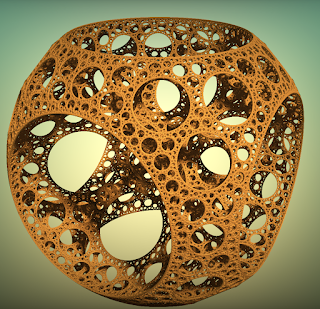
 Void-sponges are probably the easiest self-siimilar shape to make with inversive geometry, but it isn't obvious whether there is a particular shape that is somehow a better archetype than others; something that is 'the canonical inversive void-sponge'.

It does exist and there are six of them. The trick is to realise that the most symmetric 3D structure is a 3-sphere, and that regular polychora (4D polyhedra) have evenly distributed vertices on the 3-sphere.

We therefore run the iterative inversions in 4D with sphere inversion centres at the polychora vertices, then stereographically project them back into 3D. This projection is conformal and Mobius so spheres remain as spheres. Any such projection will do, but in practice there is one that mimimises the object size by placing the pole on the face centre (farthest from the vertices), this also has rotational symmetry in 3D so is the best choice. Noting that it is structurally the same shape regardless of the Mobius transformation, and these inversive shapes should always be considered as equivalence classes under not just similarity transformations but also Mobius transformations. 

So the six shapes come from the six regular polychora, the 5-cell:

The other free parameter is whole number n where the intersection angle between spheres is 180/n. For large n we get sparser shapes like above. And for smaller n they are thicker like below.

There is also the 8-cell:

16-cell:

and the 24-cell:

and here is as dense as the 24-cell gets before it encloses a sphere:

The 5-cell and 24-cell are special in that they are their own dual. A consequence of this is that you can fit another copy of the shape interwoven in it but not intersecting:

5-cells:

we can manipulate the Mobius transforms to make them the same shape in 3D:

24-cell:

and again transformed so they are the same shape in 3D:

here's a thinner version:

These shapes are not new I'm sure, but I am glad that at least one of the 49 classes of self-similar shape has a definitive family of archetypes.

Pareto Olympic Results

Olympics time, and once again we see every news site in the country splash up the medals table. Invariably with USA or China at the top. The intention is clear that the top of the table are better at Olympics in some way. Sites might even refer to the top of the table as the Olympics winners.

This is unfortunate for two reasons. Firstly, there is no the medals table. Most of the world sort by golds, then by silvers then by bronze. Parts of the US sort by total medal count (for obvious reasons). The New York Times has suggested a weighting were one gold is worth two silvers, which is worth two bronzes. 

The reason there is no one ranking is that the Olympics does not recognise any ranking table, not does it recognise a winning country. It only recognises medals to individuals. The ranking tables are not any official part of The Olympics, they are something pushed by the media, who presumably are more interested in political rivalries.

Anyway, the bigger reason this is unfortunate, is that total medals is an exceedingly unfair way to rank performance of a country. Tuvalu would need 30 thousand times the rate of medals to get the glory of matching the US on the medals table. Even larger countries like Iceland would need 900 times the rate of medal winning. The figures are even more skewed when compared to China. So why doesn't the media do the obvious thing and report medals per capita in the ranking tables?

We can get a clue by looking at the last five winners of the medals per capita (I'm using the NYT weighting here but it doesn't make much difference):

Dominica, San Marino, Grenada, Grenada, Jamaica

These are all very low population countries, and the winner varies a lot each Olympics. The problem is two-fold. Firstly, low-population countries will have far higher variance in their medal count than large ones, so the 'lucky outliers' will be small countries, and big ones like China would stand no chance of winning even if they have about the same quality of athletes, due to the lower variation.

Secondly, while this may seem unfair, the fact is that having the larger countries at the top of the table pleases more people, and so as a method is supported by more people. I'm sure that San Marino people would love to see the medals per capita plastered over the media, but their opinion is drowned out by a bigger market of people from the US and China who enjoy seeing their own country near the top.

So we are being pulled in two directions. Logic and fairness pulls us towards publishing the medals per capita, but popular interest and lucky outliers pulls us towards showing the total medal count.

This is a multi-objective problem, which can be resolved using the concept of Pareto fronts. The nice thing about this is that it admits multiple first-place 'winners' and multiple second places etc. None of these several winners can claim to be better than any other, so the slightly oppressive nature of placing every country in the world into a pecking order is relieved.

Anyway, here is how it works. In my case I will use the NYT medal weighting as the 'medals' count. The Pareto winning countries are those on the Pereto front of the two objectives: medals and medals-per-capta. They are the countries that: have more medals or more medals-per-capita than every other country.

So for any two Pareto winners, either can claim superiority to the other on one objective only, so it is a tie.

In order to get Pareto second place, we just remove the Pareto winners and apply the same search again. Likewise for third and fourth place, etc.

For 2024's Olympics we have:

• Pareto first place: Dominica, Saint Lucia, New Zealand, Netherlands, Australia, France, United States
• second place:   Grenada, Bahrain, Georgia, Hungary, Great Britain, China
• third place:    Slovenia, Jamaica, Croatia, Norway, Sweden, South Korea, Italy, Japan

Here are the Pareto first place countries in the three previous summer Olympics:

2020: San Marino, Bermuda, Bahamas, New Zealand, Netherlands, Australia, Great Britain, Japan, Russia, United States

2016: Grenada, Bahamas, Jamaica, New Zealand, Hungary, Netherlands, Australia, Great Britain, United States

2012: Grenada, Jamaica, New Zealand, Hungary, Australia, Great Britain, Russian Federation, United States

They are in population order. The table now is satisfying for people from large and small countries. 

We can see that the usual hegemony of US/China is replaced by a hegemony of New Zealand, Australia, Great Britain, and United States. Also with winning by Grenada, the Bahamas, Netherlands and Russia. 

It is actually rather sad to see that there is still Anglosphere privilege throughout the Olympics, and it isn't as egalitarian as the Olympic Committee (and the world) would like it to be. But at least now this hegemony is visible, it is not just USA battling it out with China.

Media companies would do well to present the Olympics this way. It shows what is really going on, and gives honour to some of the smaller countries with incredible rates of medals.

Update: This is a different attempt to solve the same problem with total medals and medlas-per-capita by trying to find a happy medium between the two extremes. I don't think it is the best answer for a few reasons- 1. it rates all medals the same regardless of colour, 2. it uses a model that is at the same time too complicated for audiences to adopt and too simple to represent what's going on. For instance it assumes all actions are independent. 3. it continues to squeeze all countries onto one strict ordering, rather than treating the medal rates of tiny and huge countries as effectively incomparible. 

Mixed Fractal Surfaces

It is possible to have a fractal surface which varies in local dimension everywhere. That is to say, on any patch of the surface you can zoom into a rough area (e.g. 2.5D) or zoom into a smooth area (2D). 

Here it is applied to the sphere tree fractal:

and to the non-rotated one:

In both cases the the smaller spheres are disproportionately smaller than in the usual shapes, giving a surface that tends to smooth in the vicinity of each sphere base. 

However, if you zoom in on those smooth surfaces enough you will find a sphere, and if you zoom in on that sphere enough you will find a bud at the top which is just as rough as one of the pictured ones. 

This is much like the Mandelbrot set, which has areas that are locally smooth, in the sense of being a straight thin line as you zoom in further:

But everywhere you can find tiny minibrots.

We can do the same thing with the tree surface fractal:

The surface tends to smooth, however, each smooth dome has child domes that can be just as protruding as the largest ones. So we get a mixed dimensionality. 

Because the mixture of roughnesses is everywhere and at every resolution (rather than separated) these are probably all multifractals, though I've never fully understood the definition of these. 

Scale-based decompositions

There are several ways to decompose a smooth function. A spline, a Fourier decomposition, a Taylor decomposition per-point, and a Pade decomposition per-point, are the first that come to mind. Also a perceptron (Sigmoid decomposition). 

All of these are suited to smooth functions. However nature isn't smooth, and tends to exhibit scale-symmetric roughness in some form. Can we extend some of these useful decomposition methods to support roughness?

The way I'm considering doing this is to treat scale as like another dimension. For example, if our function is 1D: $y = f(x)$, then a new axis $s$ represents scale.

As scale is a logarithmic sort of attribute, we have to treat it as such. We treat the function f(x,s) as the convolution of f(x) with the Gaussian $g(x) \leftarrow N(0,\exp{s})$, and whenever we take the partial derivative $d$ with respect to $s$ we use the logarithm: $\log{|d|}$. The modulus operation is because the logarithm is a function on the magnitude of $d$, representing the entropy of $d$. 

This $\exp$ and $\log$ pairing linearises the scale component of the function.  

We can now do something like a 2D Taylor decomposition of the 2D graph with respect to $x$ and scale $s$. This is a sort of partial derivative that can be looked at in a systematic way:

$f(x,s)$ is the height of the function (mean height of the patch)

$\frac{\partial f}{\partial x}$ is the gradient of the function

$\frac{\partial f}{\partial s}$ is the change in (mean) height with change in s, which is zero

So far not very interesting. But we can go further:

$\frac{\partial^2f}{\partial x^2}$ is the curvature of the function with respect to $x$

$\frac{\partial^2f}{\partial s^2}$ is the change in $\frac{\partial f}{\partial s}$ with scale $s$, also 0

$\frac{\partial^2f}{\partial x \partial s}$ is the change in gradient with respect to scale $s$

Now normally this last one would also be zero, but we are using the absolute value of $\frac{\partial y}{\partial x}$, so it is $\frac{g(x)\star\log{|\frac{\partial y}{\partial x}|}}{\partial s}$, which represents how much the average absolute gradient changes with scale $s$. 

This is non-zero because larger $s$ (lower-pass signals) has lower mean absolute gradient than high-pass signals for rough functions. This is a way to measure the fractal dimension of the function, since it is the slope of a log-log function. It is only non-zero on rough surfaces, and zero on smooth ones. 

This may not seem interesting, but it is starting to incorporate fractal functions and smooth functions into the same framework. This is a sort of Taylor expansion at a point, but it can also be applied piecewise as the basis for approximating a whole 1D function. We can now treat a function as a set of heights quadratically interpolated, and each with their own fractal dimension, so they are rough curves. Moreover, this piecewise decomposition is a mesh in 2D with scale s, giving a different set of slopes and fractal dimensions at different scales. 

This is already very powerful, it supports roughnesses that change with location and with scale. Moreover we can see a link with splines, since piecewise linear approximations are first-order splines. But we can keep going:

$\frac{\partial^3f}{\partial x^3}$ is the rate of change of curvature, used in cubic splines for instance

$\frac{\partial^3f}{\partial x^2 \partial s}$ is the change in curvature with scale, I think this quantifies a C(1) fractal, representing not rough but lumpy functions. However I'm not sure!

$\frac{\partial^3f}{\partial x \partial s^2}$ is the change in fractal dimension with scale. Does it get rougher or smoother as you zoom in. This is connected to my Saturated shapes blog post.

$\frac{\partial^3f}{\partial x \partial s \partial x}$ how the fractal dimension changes with $x$, this allows linear roughness changes along the function. 

$\frac{\partial^3f}{\partial s^3}$ this is zero 

This next level of Taylor expansion can characterise the curvature of the function and the change in roughness.  

 

 There are lots of ways this idea could be extended:

• Look at Pade decomposition instead, or Fourier decomposition
• Extend to a 2D function (like a hillside), this adds many more partial derivatives
• Look at the topological groups instead, e.g. -ve, 0, +ve in each component of the Taylor expansion 

For the 2D case:

$\frac{\partial^2f}{\partial x \partial z}$ - twist or saddleness

$\frac{\partial^3f}{\partial x \partial z \partial s}$ - very weird idea, how much does saddleness change with scale 

$\frac{\partial^3f}{\partial x \partial s \partial z}$ - how much does $x$ fractal dimension change with $z$. Noting that roughness can be different in different axes

We can then have a linear sum of all of these primitive values. Topologically we we can set each to -1,0 or 1, to give us a set of derived shapes.

 

 

 

 

 

 

A tree-solid

A tree-solid is a scale-symmetric shape which is a tree (acyclic, no holes) but fills the full area of space.

It is the set complement of a void-tree which is what we usually call fractal trees. So people usually just make fractal trees like the Vicsek fractal:

But making one primarily as a tree-solid makes you consider the shape of the solid regions it is built off. In the case of this post, it is disks.

To make a tree from disks they must overlap, so the shape is an overlapping disk packing, with the overlaps in a tree topology.

If is possible to make it with any intersection angle between the disk and its parent, but I used 90 degrees, which is half way between the two extremes:

You can probably just make out the disks that it is build from.

Another way to arrange part of this structure looks more like the Vicsek fractal:

To see the circles more easily in the first image we can colour them according to which iteration they were on:

Same for the second variant:

which can be rotated:

The reason I made this structure is that I'm looking into whether there is a 3D equivalent. This would be a tree-solid, or visualised as its complement: a void-shell. This is a lot harder to make, and may not be possible.

FYI, the limit of both of these variants as the intersection angle decreases to zero is the non-overlapping disk packing here:

 

A democracy problem

This idea follows from my last post about dinosaurs funnily enough. It relates to a common problem in democracies called the tyranny of the majority. This may sound like a strange term because surely having a government that reflects the majority opinion in a country is a good thing. But in fact it is problematic.

Let's take an example where 60% of a country is Christian and 40% is Muslim. In one general election we would expect a party with Christian-aligned policies to gain power. This is a reasonable outcome for a single election.

But over the period of 100 general elections, there is a good chance that all of them will be won by a Christian-aligned party, since 60-40 is a very large majority in politics. This leads to frustration by the minority population, disillusion, and instability.

The problem hinges on the fact that:

mean({a,b,c,..}) ≠ {mean(a), mean(b), mean(c), ...}

Where mean() and a,b,c can refer to many more aspects of democracy. For instance, mean(x) could be 

• the winning party in electorate x. 
• the elected party for each election year x.
• majority vote for each bill x.

In each case the fallacy is that a set of "mean" opinions is sufficient to be a mean set of opinions. 

But these are not the same thing. A set of mean opinions lacks the diversity that should exist in a mean set of opinions. 

For example, if each consistuency has a range of views on retirement age from 55-75, with the mean at 65, then the MPs representing the mean view of the consituencys will *all* vote for 65 as the retirement age. It will appear as though the country is united. If you are a subculture that occupies 10% of the vote wanting a retirement age of 55, none of the 200 MPs will be representing your view.

Ideally, a mean set of retirement ages that reflect the constituencies should have a diversity of views from 55-75. And a correct mean set does indeed reflect this diversity. But you cannot calculate it just by taking the set of the individual means.

It is interesting that this problem has been acknowledged, and some countries, such as New Zealand, use proportional representation to alleviate this problem. In this case 10% of the MPs will reflect the 10% of the population supporting 55 year old retirement. 

When the proportion is the same across districts, this is exactly what the 'mean set' gives (see last post), for distinct classes like parties, where the mean naturally becomes a mode.

However, when the proportion varies across districts, we get something different to standard proportional representation. 

For example, what if the proportion of a and b are 20% and 80% in France and 60% and 40% in Spain, and your representative set is one from element from France and one from Spain?

In this case, if the order is France,Spain then (a,a) has chance 0.12, (a,b) has chance 0.08, (b,a) has chance 0.48 and (b,b) has chance 0.32. Then with order symmetry, the chance of {a,a} is 0.12, {a,b} is 0.56 and {b,b} is 0.32. So {a,b} is the mean set. This is different than if we just added up all the probabilities to give 40% for a and 60% for b, then you would get 0.48 for {a,b}.

This is a proportional representation of the views of each of the constituencies, rather than a proportional representation of overall votes. It includes the individual constituency view back into the result. 

There are a million different PR schemes, so it would be interesting to see if this is one of them, or how it compares.

As mentioned in the bullets earlier, it would also make sense to use mean sets over multiple general elections. So if one party always gets 10% of the vote then over 10 elections it will get in once.

Mean dinosaurs

There is a phenomenon about dinosaurs that seems interesting to explore. If you look at a poster of dinosaurs you'll notice that none of them have wattles, or extreme features like peacocks, or trunks or frill-necks or fleshy crests. In fact none of them are old or have a broken arm, none are overweight or missing a limb etc. This is odd because you would expect to see these characteristics occasionally, but in a collage of 100 dinosaurs you don't see any.

What's going on is that each dinosaur is individually reconstructed to be the best estimate from the data, moreover, each archetype is chosen to essentially be the average of all individuals of that species. So it has average age, average weight, and from our knowledge of that species it is unlikely to have any of the unusual features, so these are left out. Let's use the word mean(x) to be this best-guess average for that species.

This is well and good for the individual species, but when we present a set of dinosaurs we can't just use the mean for each species. We unconsciously ignore the fact that: 

mean({T-rex, triceratops, diplodicus, ..}) ≠{mean(T-rex), mean(triceratops), mean(diplodicus), ..}

An average set of dinosaurs is not the same as the set of average dinosaurs. I'll show that this is related to averages over spaces with symmetries, so putting it in the same category as my previous 'mean xxx' posts.

Height

To explore this, let's start with a simpler case, a single species T-rex and a single characteristic, such as height. If we want to represent a single T-rex then using its mean height is the sensible choice. OK maybe we should use the modal height, or median height, or some other average, but for simplicity let's just use means. The same ideas apply, probably more so, for the other, less linear averages.

If however we want to show a set of two T-rex's, then both having mean height is not the average height distribution for that set. 

Here the mean height is 175cm (not a real T-rex! diagram from google) and the distribution of heights is approximately normal, with one standard deviation being 7 cm. 

It might be tempting to think that if you sample two T-rex's from the distribution, they will have on average heights 168 and 182 cm, i.e. plus and minus one standard deviation. This is not right.

You might also choose the two points shown in dark red, which are the half-way area points for the top and bottom half of the normal distribution. These are roughly 0.7979 standard deviations. This is also not right. 

The way to solve this is to take the 2D distribution of the two T-rex heights, and note that the two T-rex's are interchangeable, so rather than a 2D Euclidean space, it is a topological space with reflection symmetry on the diagonal; it identifies point pairs (x,y)=(y,x). This is a valid space on which to find a mean 2D point:

Here we see the 2D normal distribution for the two dinosaur heights, and the mirror symmetry down the magenta diagonal. As a consequence of this symmetric space, the mean 2D point is shown in magenta. Its value is sqrt(0.5) of the mid-area value, which is 0.564 standard deviations:

If we had three T-rexs on our poster then the mean set of heights could be found in a similar way by taking Euclidean space R3 but with the order symmetries (x,y,z)=(y,x,z)=(x,z,y)=(y,z,x)=(z,x,y)=(z,y,x).

In general can calculate the height for n T-rex's by sampling an n-dimensional normal distribution, sorting the elements in order, then taking the average over all ordered samples. Here are the sets for n = 1 up to 5, in standard deviations:

n:

1 {0}

2 {-0.564, 0.564}

3 {-0.84, 0, 0.84}

4 {-1.03, -0.297, 0.297, 1.03}

5 {-1.16, -0.495, 0, 0.495, 1.16}

You would of course multiply these by the standard deviation and add the mean, in order to get the correct mean set of T-rex heights.

Additionally, this approach is not just for normal distributions, it can apply to any distribution.

Height and width

What if we have two characteristics? For a single T-rex we simply use the mean height and mean length identified for that species. For a set of two T-rex's we have a 4D distribution function. The height and width are clearly interdependant characteristics, so is not just the product of the two individual distributions. That is fine. 

We then introduce the ordering symmetry (xh,xw, yh,yw) = (yh,yw, xh,xw), and find the mean 4D point, which is the weighted mean coordinate, weighted by the probability density at each coordinate.

At this point things get interesting. A mean on a non-Euclidean space is a different sort of beast. You can find it by randomly sampling the (4D) probability distribution, then choosing the closest ordering to the running average before adding it on. For the 2D case above this tends to a single result (or its reverse ordering), in 4D there is a remaining symmetry, that gets broken by this process. The result is a mean 4D point that changes each time you find the mean value.

As a result, your mean value (representing a set of two T-rex height and widths) itself follows a distribution. 

When the two distributions are uncorrelated and equal, the mean set is a uniform circular distribution around the mean, of radius 0.564, offset 0.564(sin a, cos a) with the other dinosaur in the set having offset 0.564(-sin a, -cos a). With a resulting from spontaneous symmetry breaking to a different angle each time the mean set is calculated.

If the two distributions are correlated, then the mean set distribution will be non-circular, and in fact elliptical if the distributions are a simple multivariate Gaussian. For highly correlated characteristics this random angle a will tend to give an offset in the long axis, giving consistent results each time it is calculated, in particular:

If height and length are positively correlated (as they usually are) then the distribution of means clusters around a set which is one short,narrow T-rex and one tall,wide T-rex. 

If height and length are negatively correlated, then the distribution of means clusters around one short, wide T-rex and one tall,narrow T-rex.

If there are three T-rex's in the set then the mean set still is a distribution over the (width,length) direction angles. But unlike the single-characteristic case, the three (width,length) vectors are not in a line. For equal unit sigma Gaussians, a calculated mean set is {(0.33,0.707), (-0.78,-0.06), (0.44,-0.647)}. This distribution of the variation onto the 3 dinosaurs is rotated each time it is calculated, with the sum of the squares of the values always being 1.84. These three points, as you might have guessed, form an equilateral triangle.

Above: width,height values for set of 3 T-rex's, with the standard deviation for the covariance in red.

In general, the mean set of m characteristics for n T-rex's distributes the n points over the m-dimensional ellipsoid of the distribution (or other shape), up to a rotation in m-dimensional space.

Species

Instead of characteristics, what if we have a known list of species with probabilities of occuring, and we wish to represent that as well as possible with a set of just two dinosaurs?

For independent classes like this, we have to use the mode rather than mean value. This is not just a big change, we already have integer means that round to the nearest integer, and integer weighted means. The mode is just a weighted mean like this, but for the n classes placed at the corners of an n-simplex.

Imagine the probability of spotting a T-rex is 50% and a triceratops is 50%, then to find the modal set {a,b} you have four possibilities: {T-rex, T-rex}, {T-rex, Triceratops}, {Triceratops, T-rex} and {Triceratops, Triceratops}, each with 1/4 likelihood.

But the middle two are equivalent in a set, so the {T-rex, Triceratops} set has twice the likelihood of the other two. 

This means that the modal set is {T-rex, Triceratops}. 

Even if the percentages are 66%, 34%, the modal set still contains one of each. Any fewer Triceratops and the modal set would be just two T-rex's.

For sets of three from two dinosaurs you have the options {a,a,a},{a,a,b},{a,b,a},{a,b,b},{b,a,a},{b,a,b},{b,b,a},{b,b,b}. But with the order symmetry there are only: {a,a,a},3{a,a,b},3{a,b,b},{b,b,b} with the relative likelihoods expressed with those coefficients. As a result now even if the Triceratops has probability 25.1%, it will appear in the set of 3 dinosaurs. 

Above: relative proportion of T-rex (b) with the mean set below it. 

This generalises to n set elements using the Pascal's triangle pattern. The result is that the sets distribute evenly over the possible relative proportions of the two dinosaurs. 

If there is a third dinosaur involved, and the mean set has three elements, then they have the following weightings: 1{a,a,a},3{a,a,b},3{a,b,b},1{b,b,b},3{a,a,c},3{a,a,c},1{c,c,c},3{b,b,c},3{b,c,c},1{c,c,c},6{a,b,c}. The result of this weighting is that the sets distribute evenly over the space of relative proportions of the three dinosaurs, which is a triangular space:

The mean set is therefore a proportional representation of the dinosaur weights. I fully expect the generalisation to n dinosaurs and m members of the set, to be a proportional representation.

Species with characteristics

What if we have a T-rex with a height distribution and a Triceratops with a different height distribution function? This becomes a hybrid of the discrete and continuous methods. 

First we look at the total probability (the area under the probability density function) for the two dinosaurs. These are our probabilities that will decide whether the mean set will be {a,a}, {a,b} or {b,b}. 

Then, let's say it is {a,b} and heights x,y, we generate the 2D probability distribution function P(x,y) = Pa(x)Pb(y) + Pb(x)Pa(y)   (the sum here due to the {a,b}={b,a} symmetry).

The centroid of this combined probability distribution gives you the height of the dinosaur a (x) and dinosaur b (y) to give the mean set {(a,x), (b,y)}. However, this mean set is itself a distribution, with some percentage also being {(b,x),(a,y)} depending on the relative total probabilities in the sum above.

If the T-rex is usually tall and the Triceratops usually short, then this will give an essentially singular mean set {(T-rex, tall), (Triceratops, short)} as expected. If they have the same distribution then there are two equally possible mean sets {(T-rex,mean+k),(Triceratops,mean-k)} or {(T-rex,mean-k),(Triceratops,mean+k)}.

General characteristics

If dinosaurs characteristics are highly correlated to their species, then your representative set mean{a,b,c} really is close to {mean(a), mean(b), mean(c)}. For example, if it was a microraptor, T-rex and brachiosaurus and the characteristics were height and neck length, then the set {mean{microraptor}, mean{T-rex}, mean(brachiosaurus)} is representative.

If however the characteristics are more uncorrelated with the species and with each other, then the mean set itself has a distribution of values, and your best strategy is to sample one at random. This is the case for things like 'contains a wattle', 'is overweight', 'is old', 'has a broken arm'. They all could happen to any species, and are uncorrelated with each other. 

So in this case your pair of dinosaurs should sample at a calculated k (Mahabolonis distance) from the mean, and produce the pair which are the equal and opposite from the mean in this random direction. 

Generalising to n dinosaurs in the set, the n dinosaurs sample n representative points in terms of sigmas (Mahabolonis space) from the mean, in a random direction.

This mean that sets of dinosaurs recover the variety of characteristics that are not evident in the {mean(a), mean(b), mean(c), ...} set.

In Short

Anyone who depicts a representative set of dinosaurs by using individual mean dinosaurs, is only correct when their characteristics are strongly correlated to the species and with each other. 

For more uncorrelated characteristics, larger sets are increasingly poor representations, and lack the diversity that they should show. 

We often see posters of dinosaurs where they are all the same age, all uninjured, none with unexpected fleshy features, etc etc. This all comes down to missing the key fact that:

  mean({a,b,c,...}) ≠ {mean(a), mean(b), mean(c), ...}

Mean Transformations

A while back I looked at mean polyhedrons and said that the mean cuboid should have sides of length (2,5,11) or (1,2.5,5.5).

A different way to estimate a shape's principle dimensions is to represent it by a random transformation of a sphere by a transformation matrix M. The eigenvalues of that transformation then give the principle dimensions of the resulting ellipsoid. This can be done in any number of dimensions and just requires a decision on what a random nxn matrix should look like. 

If seems to me that what I should really do is treat it as a n^2 length vector with equal likelihood of pointing in any direction. This is easily achieved by sampling each vector element from a N(0,1) normal distribution, then normalising the vector.

I then order the eigenvalues by their absolute value and average them over 300,000 randomly sampled vectors representing the matrix M. The resulting shape dimensions for each number of dimensions is:

1: 1

2: 1, 2.34, 

3: 1, 2.70, 4.41 

4: 1, 2.393, 4.23, 6.04

5: 1, 2.532, 4.096, 6.130, 8.16

6: 1, 2.412, 4.06, 5.67, 7.77, 9.90,

7: 1, 2.486, 4.02, 5.774, 7.475, 9.705, 12.0

8: 1, 2.417, 4.00, 5.557, 7.35, 9.084, 11.371, 13.731

9: 1, 2.464, 3.99, 5.65, 7.27, 9.14, 10.95, 13.33, 15.82

10:1, 2.420, 3.98, 5.524, 7.214, 8.856, 10.756, 12.61, 15.04, 17.61

A few interesting things to note:

1. The pattern is not simple, the second extent for example oscillates, perhaps converging towards 2.44 somewhere.

2. The third extent however just decreases, converging towards 3.95 perhaps

3. The fourth extent also oscillates, the fifth decreases and the sixth oscillates... do only the even extents oscillate?

4. They all seem to converge, suggesting that there is a value for the infinite dimensional shape. 

5. The shape is quite different to the previous mean ellipsoid for the 3D case. That one was more cylindrical, this one is more planar.

6. For each dimension the sequence grows superlinearly. Is there a pattern?

If we look at the difference between consecutive extents in the 10D case:

1.42096, 1.55935, 1.54375, 1.68965, 1.64261, 1.89974, 1.85389, 2.43466, 2.56585

You'll notice that this is also not smooth, it oscillates, though this time while growing. The same is true for all cases < 10D too. So none of the extents seem to follow a simple pattern.

Update: this topic seems to be exactly the subject of Random Matrix Theory, and the above eigenvalues should tend to a semicircle distribution if I'm understanding it right. The oscillations appear in the link for finite values of n (probably causing the oscillation with respect to n too):

 The simple takeaway is that as n tends to infinity, the distribution of Eigenvalues will tend to a quarter circle (or a semicircle if we allow negative eigenvalues). This semicircle histogram is because the eigenvalues (in the complex matrix case) tend to a uniform unit disk distribution.

Saturated and desaturated 3D shapes

Saturated

Here are some more examples of saturated shape (see last post), this time 3D. I've used the inversion sets table as a starting point.

These saturated surfaces all have fractal dimension 2, so they are 2D surfaces. However their surface areas are infinite. A measurable area needs to be in m^2 log^n m where n is larger for the lumpier shapes:

These are also saturated surfaces, but this time saturated with spheres rather than lumps or dents:

Neither are fractals and neither have finite surface area. 

These curves all have fractal dimension 1, they are non-fractal (branching) curves, however their total length is infinite. You need to measure their size in m log^n m for some n representing how saturated they are:

(ignore the sphere in the centres of the last one, an artifact of too few iterations)

This set is disparate points, or dust. It's fractal dimension is 0 like its topological dimension, so it is not a fractal. But the number of points is infinite, you need to 'count' the points in log^n m:

So saturated shapes are relatively easy to create in 3D. 

All of these shapes are nowhere differentiable. They are more lumpy than C(1) fractals like the Hevea project shapes which are differentiable and also have finite length/area.

Desaturated

This is a desaturated tree surface fractal. Its fractal dimension is something like 2.5, but the roughness grows at the finer details, such that its area in m^2.5 is zero. 

Here is an equivalent with the cluster-tree fractal:

 

In both cases the desaturated shapes look sharp compared to the rough fractals, and the saturated shapes at the top look blunt.

Here's a desaturated shell-shell:

The equivalent for the void-tree again has most of the geometry at the finer scales:

Saturated and desaturated shapes

Here's an unusual curve:

Its fractal dimension is 1, so it is not a fractal. But its length is infinite. It is constructed like a Koch/Cesaro curve with local dimension D(i) at iteration i given by D(i) = 1+1/i. Where the per-iteration bend angle equals 2asin(exp(-ln(2)/D(i))).

The question is how do you compare the lengths of different subsections of the curve, if they're all infinite? This is reminiscent of the Coastline paradox. 

There are related curves that have local dimension D(i)=1+0.5/i and 1+2/i respectively:

This raises a second question, not only do we not know which is longer, but they clearly change in how lumpy they are. How do we measure that? 

I described them all as lumpy, rather than 'rough' like fractals because the lumps are only at the larger scales. I use the term saturated to describe these curves. Their length has saturated to infinity and it also invokes the idea of a shape saturated and swollen with water like wrinkly fingers in the bath.

This next curve has local dimension D(i) = 1.2618+1/i so it is a fractal, in fact it is the saturated version of the Koch curve. Its fractal length (fractal content or Hausdorff measure) is infinity.

Moreoever if you measured this fractal content for a slightly higher dimension such as 1.2619, it would be zero. So you cannot use fractal content to measure the length of this curve either.

The answer to these problems is that instead of measuring these lengths in metres (or metres^1.2618 for the saturated Koch curve) you measure the in m log^n m (or m^1.2618 log^n m respectively). In general any shape of dimension d that is saturated can be measured in m^d log^n m. Here n is the value that describes their lumpiness. In these examples when the local dimension is D(i) = D + k/i, then n = k ln(2).

The shapes don't have to be curves. This is a particularly pure case of a saturated 0D shape, i.e. a point or finite number of points, where D(i) = 0 + 1/i:

There are infinite points in this saturated shape, but unlike the 2D Cantor set its fractal dimension is still zero, so it is not a fractal. But, you can still compare the size of these shapes (or portions of them) as they can be measured in log^n metres. Here is a twice as saturated set of points (twice n): D(i) = 0 + 2/i:

The point spacing is decreasing as we zoom in. Indeed all of the above examples change their scale and shape as you zoom in. But even though their log-log plots are curved it is still possible for shapes to be scale-symmetric. Take for instance these binary trees:

They both have fractal dimension 1 so are not fractals, just connected lines. If the stem length is 1m then the left image has total length 12 m. But the right shape has infinite length; it is saturated. We can still measure its "length" as 2.88 m log m. This saturated tree occurs when the child branch lengths are exactly half the parent branch length. 

Desaturated shapes

The same thing happens in the other direction. You can take a 2D area and remove the harmonic series. Here the local dimension is D(i) = 2 - 1/i, and 2 - 2/i respectively. They both have area zero, so how do we compare their sizes?

Similarly you can also desaturate a fractal, such as the Koch curve here, using D(i) = 1.2618 - 1/i. Its fractal content is then zero.

The equivalent measurement for these is to measure in m^d / log^n m.

Here's a desaturated solid triangle, with D(i) = 2 - 1/i:

I call these desaturated as their d-volume has all of its size "dried" out of it, like dried ground that has split. In general we can think of these desaturated shapes as dessicated or depleted versions of the original shape.

This next shape is a line using a binary subdivision formula with D(i) = 1 - 1/i:

It looks like a Cantor set but its fractal dimension is 1 and its 1D length is 0. You must measure the size of this desaturated line in m/log^n m.

These aren't the only shapes that act this way. If we plot the box counting dimension of the boundary of the Mandelbrot set as a log-log graph, then we plot the function y=-2(x-s) - g log_2(-(x-s)), we see that it fits quite well to the curve when s=18.6, g=3.8:

This function when translated to a gradient error with its fractal dimension of 2, is also a 1/x harmonic function. The close match is suggestive (but certainly not proven) that the Mandelbrot set's boundary is also a desaturated area, with n equal to g. This would explain some previous suggestions that the boundary's area may be zero despite it having dimension 2.

Above: compare the outer Mandelbrot boundary with the next largest minibrot to see how much denser the boundary gets as you zoom in. (image thanks to Claude). 

If the above function is close then you can convert it to the physical quantity formula by replacing x with ln(1/x) and taking 2 to the power of y. The resulting formula tends to m^2 / log^n m for large x, giving the size of the Mandelbrot set boundary as: 3026 m^2 / log^3.8 m.

But we don't know that the function needs to reach down to the 1 box level (y=0), the function only needs to be asymptotically correct (for large negative x). 

It also isn't necessary to have the same s in both parts of the formula, so with different values we can get more curvature in out best-fit curve by dropping n to 2, when s1 = 14.3 and s2 = 12.7 we get a size of:

15 m^2 / log^2 m:

If n = 1 then s1 = 12.3 and s2=9 is a good fit, so you get a size of: 1.36 m^2 / log m:

Both of these seem somehow more likely than n=3.8. But we would need more data to make a better guess on n, which describes how desaturated (dessicated) the boundary is as a 2D region. 

The function to simplify in these cases is: y=2^( -2(log(2,k/x)-s1) - g*log(2, s2-log(2,k/x))), where k is the number of pixels per unit in the image, which is 3600 for this case.