Mean points

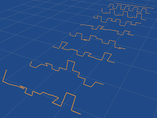
 We can also look for a mean set of points. This has continuous rather than discrete symmetries. The starting point is the 1D case: what is the mean set of repeating point locations? It depends on how many points are in the sequence, so here is the answer for the first 10 numbers of points:

The images on the left represent the sequence as the points in a circle (rendered as radial spokes). 

As you can see, the result is fairly trivial, the sequence seems to be symmetric, with a single largest gap, and progressively smaller gaps on either side of it. 

If we include reflection of the sequence in the equivalence class, the results appear to be exactly the same.

2D

We could explore the 2D case in a toroidal universe as with the previous mean textures post, but this doesn't easily allow a continuous rotational symmetry. Instead, let's look at a spherical universe, so find the mean set of n random points on a sphere. 

To do this, I need a way to find the least squares orientation between two sets of points on a sphere. To avoid the uncertainties of approximate methods (such as Iterative Closest Point etc) I compare all permutations of the points and run an absolute orientation function on each permutation (Eigen::umeyama). The R which has the smallest sum of squares difference is chosen, and applied to one set of points before averaging them and renormalising.

Unfortunately, this permutations approach is intractable for larger numbers of points, so I show here only up to 5 points. Giving just a hint of the pattern for mean points on a sphere.

2 points:  (right angle)

0.437025 0.490747 0.753775,   0.67137 0.379744 -0.63644

3 points: 

 

0.147701 -0.525988 -0.837568,   0.981211 -0.192266   0.01611,   0.104602 -0.529166  0.842047

4 points:

-0.394284 -0.910857 -0.121984,  -0.680957  0.712358 -0.169835,   -0.983752 -0.0842168   0.158555,   0.184711  0.622359 -0.760626

5 points:

-0.295731  0.738672 -0.605728,   0.690733 0.0875932 -0.717785,   -0.97845 0.0669067 -0.195341,  -0.301121 -0.657821 -0.690361,  -0.651082 -0.174766  0.738613

6 points:

0.129365 -0.627223  0.768021,  -0.434599 -0.871754 -0.226204,   0.367076 -0.768696 -0.523795,  -0.841728 -0.113547  0.527827,   0.769293  0.153797 -0.620109,  -0.778213   0.13924  -0.61237
 

These at least show that the mean set of points on a sphere does not follow a trivial pattern. The points aren't in a plane or even within a radial cone.

Mean textures

We can extend the idea of mean signals into 2D, as mean textures. In the previous post I found two signed and two complex signals that were non-trivial (they didn't tend to a spike signal). Here I look at the case for 2D, on signed textures (greyscale with 127=0). 

Here are the results with no 90 degree rotational symmetry. Showing a 5x5 tiled patch from a 2x2 texture (left) up to a 5x5 texture (right):

If I include reflection when matching:

If I include 90 degree rotational symmetry (no reflection):

And with reflection included:

Finally, for comparison, here is an unsigned texture, with 90 degree rotational symmetry, no reflection:

The unsigned texture is just like the unsigned signal of the previous post. The mean is a single spike. For the signed textures, they all appear to tend towards a pair of extremes (one positive, one negative) as the width goes up to 5.

One reasonable variant is for the random values to be a uniform distribution of signal energies (value squared). This supports the need for negative values, since we are taking the square root of the uniformly sampled numbers.

Here is with no reflection: (28 iterations)

 

and with reflection (28 iterations):

These do not show the same tendency towards a trivial case of one or two spikes at larger resolutions. However, the accuracy of the 5x5 is very poor, due to the huge number of iterations needed to converge. The rest are quite close, as verified by trialing with different random seeds.

Here's the above 4x4 (no reflection) shown over a larger surface:

We also do something very similar in the complex domain. Here I use the red component for real values, the green for imaginary values and set the blue to halfway. Lower iteration count (23) just to give an indication of what it might look like:

without reflection:

with reflection: 

Mean signals

Here I look at the average of discrete repeating signals. That is, I pick random signals (by sorting a random set of values between 0 and the signal length, and using the differences). Then I match the signal to the running average using a cross-correlation, by sliding in time, and optionally reversing the signal direction.

Here are the sequences visualised, from length 1 to 10. One grid cell is 2 units high.

no reflection                                        reflection

We can also include negative numbers. Each candidate sequence has a sum of absolute values equal to the sequence length. A cross-correlation works equally well, but we can also choose whether to allow negation of the values when matching. Here grid cells are 8 units.

1,3: no reflection, 2,4: reflection. 3,4 includes negation when matching.

A different approach is to pick random values between 0 and 1, and match based on minimising sum of square error, rather than maximising cross correlation:

left side: unsigned, right side signed. 1,3 no reflection, 2,4 allows reflection

Notice that the results get smaller for larger sequences. This isn't true for the cross-correlation, and I find the cross-correlation method more general as it represents scale-independent matching.

A natural extension of the cross-correlation on signed numbers is to use complex numbers. We cross correlate as the sum of one times the conjugate of the other, and pick the match with the largest real component.

 

left: no reflection                                    right: with reflection of signal index

There are more reflection options for complex numbers. We could also negate the value in the reflected match (below left), or conjugate the complex value in the reflected match (below right): 

 

Of the four, it looks like the first two (no-reflect and reflect) give the least trivial result.

We can also use the largest absolute value in the cross-correlation, and so 'rotate' the complex signal when adding it on. This is adding an explicit phase invariance. However, these give more trivial results:

left: no reflection, middle: reflection included, right: reflection with conjugation.

It is not clear that having an even distribution of absolute values is the best constraint on signed and complex values. It may make sense to have an even distribution of signal energy (value squared). Doing so gives results with slightly less spiking and clearer patterns:

left: no reflection, right: reflection allowed.

I have only shown signal lengths 1 up to 8, as the larger ones become too inaccurate, but the above are repeatable. The no-reflection case, shows a hint of a pattern, with the n=2, 4 and 8 cases close to square waves. and the n=3 and 6 cases being uneven square waves. As for the reflection case, it shows signs of following a saw-tooth wave until about n=6.

Mean polyhedrons

The previous post was a method to find the average polygons of a certain number of sides, assuming that one defines a polygon by its interior angles and edge lengths. 

If we just define shapes by their edge length then we can obtain average triangles and also average tetrahedrons. Without loss of generality, we pick randomly distributed edge lengths which sum to 1.

For triangle edge lengths a,b,c, we get the means (shown over 4 independent trials): 

a,b,c: 0.4, 0.2, 0.4

An isosceles triangle.

when we include reflections, we get an obtuse triangle:

a,b,c: 0.444, 0.361, 0.194

For tetrahedrons we pick 6 edge lengths, and throw out any invalid tetrahedrons. Those being any with faces that disobey the triangle inequality (sum of shortest sides must be greater than longest side) or disobey the tetrahedron inequality (sum of smallest face areas must be greater than the largest face area). 

With these remaining tetrahedra, we find the closest match (dot product of the vector of edge lengths) for all relative orientations. For tetrahedra that is 12 orientations. We convert the mean edge lengths into coordinates like so:

Under this system, the mean tetrahedron is fairly unstable, but seems to look a bit like this:

a,b,c,d,e,f: 0.157258, 0.184638, 0.178683, 0.143683, 0.16418, 0.171558
r,s,t,u,v:     0.115537, 0.144023, 0.113931, 0.035557, 0.123238

coords: (0,0,0), (0.179,0,0), (0.116, 0.144,0), (0.114, 0.0356, 0.123)

If we allow reflection when matching shapes, then the result look more like this:

a,b,c,d,e,f: 0.195577, 0.184195, 0.126073, 0.159834, 0.193624, 0.140698
r,s,t,u,v: 0.0458932, 0.178386, 0.0402287, 0.0351516, 0.130161
coords: (0,0,0), (0.126,0,0), (0.0459, 0.178,0), (0.0402, 0.0352, 0.130)     

Here it is top down: 

Cuboids

For normal right-angled cuboids, we know from the mean signals post that the mean edge lengths must be proportional to 2, 5 and 11:

This is because the cuboid has no further constraints on its edge length, and its symmetries are the same as a length 3 sequence with reflection allowed.

Mean polygons

What does a triangle look like? It is easy to give an answer, but harder to find the best answer: the triangle closest to all others; the mean triangle. The same can be asked of more sided polygons.

Here's my best effort at calculating the mean polygons:

tri: 31, 0.46, 31, 0.27, 118, 0.27. quad: 61, 0.32, 69, 0.32, 61, 0.18, 170, 0.18. pent: 233, 0.08, 70, 0.19, 83, 0.30, 83, 0.24, 70, 0.19.

We can also find the mean of just the convex polygons:

tri: 31, 0.46, 31, 0.27, 118, 0.27. quad: 63, 0.35, 79, 0.20, 109, 0.20, 108, 0.25. pent: 92, 0.32, 91, 0.16, 116, 0.19, 124, 0.18, 117, 0.16.

The asymmetry of two of these is interesting. There are of course two mean shapes in this case, one being the reflection of the other. But whenever you take the mean of this shape with its reflection, the best alignment must on average, create a new mean that looks like the mean shape again (or its reflection). That is what I assume is happening anyway.

If we allow the equivalence class of shapes to include reflections, then we get more asymmetric results:

tri: 16, 0.47, 42, 0.16, 122, 0.37. quad: 32, 0.39, 70, 0.23, 74, 0.16, 184, 0.22. pent: 78, 0.06, 244, 0.22, 57, 0.30, 70, 0.29, 91, 0.12.

And finally, the convex only mean polygons:

 

 
tri: 16, 0.47, 42, 0.16, 122, 0.37. quad: 91, 0.12, 97, 0.22, 135, 0.24, 38, 0.41. pent: 63, 0.36, 110, 0.10, 112, 0.14, 126, 0.22, 129, 0.17.

In order to find these mean polygons, we have to decide what the space of polygons is. 

In my opinion a polygon is defined by a set of interior angles from 0 to 360, and a set of edge lengths. We pick from the set of all such values which produce a valid closed polygon. In practice, we do this by choosing a random set of bearings (from 0 to the expected sum for that polygon), then ordering them and using the adjacent differences as the set of angles. This gives a uniformly distributed set of angles such that they add up to the expected total. We do the same thing for edge lengths. We then check whether the resulting polygon is close to being closed. If it isn't, we throw it out. If it is then we adjust the edge lengths to pull it together (this should only introduce a tiny error if any).

Now we can generate random polygons, we need to decide how to average them. We shouldn't just average the parameters (angles and lengths) because these are shapes, and shapes are an equivalence class. Usually, shapes remain the same shape under Euclidean transformations and scaling. So I average each pair of n-sided polygons together by comparing against all n relative rotations and taking the sum of the products of the interior angles, and multiplying it by the sum of the products of the edge lengths. This is a form of cross correlation, and the greatest match defines how one polygon is rotated relative to the other. We take the mean of the polygon parameters once they are matched (shifted around the loop to be as close as possible). We therefore take the mean of pairs, then take the mean of pairs of these, and so on. The reason I don't just accumulate a running mean, is that I don't want symmetry breaking, where a particular bias then is strengthened.

 

Fourier-Mellin Fractals

The Fourier-Mellin Transform (FMT) seems to be fundamental in encoding 2D fractals.

Here are example kernels of which the FMT composes all shapes:

Notice that these are standard Fourier transformation planar waves, but in log-polar space. Also notice that these are basic components of shapes with single scale symmetry (an image that is invariant to a single similarity transformation), you can build any sort of scale-symmetric spiral from summing these.

If we take a 2D image I:

and get its Fourier transformation F(I) then all shapes in any location will produce the same abs(F(I)):   (zoom in on centre to see):

Now, if we take the log of this log(abs(F(I))) (as though it were on a complex plane), i.e. convert to log polar coordinates: (horiz = angle, vertical = log radius from bottom to top)

The result is vertically periodic only if it is a broad class of scale-symmetric shape. (Above we see the lines getting softer towards the bottom, that is just because there aren't enough pixels close to the abs(F(I)) centre to represent the low spatial frequencies of the red squares shape. The precise result would be periodic).

The height offset of the vertical translation symmetry represents the scale involved in the fractal. In this case it is scale=2.

Next, we take the Fourier transformation of this, and get its absolute, to give the Fourier Mellin Transformation: FMT = abs(F(log(abs(F(I))))):

This gives an encoding of the shape that is now invariant to rotations and scalings.

Let's do it again, this time with a Menger sponge...

                      I                                      abs(F(I))                       log(abs(F(I)))      

                                               FMT = abs(F(log(abs(F(I)))))

and with the 2D Cantor set:

                                   I                                                 FMT(I)

As you can see, the Fourier-Mellin transformation is different to the squares examples. The intermediate images are hard to see, so you'll need to zoom in or brighten them to see better.

Now, this FMT is invariant to translation, rotation and scale. To illustrate, here is the FMT calculated for the Viscek fractal at two different scales and rotations:

     

Not only does the FMT represent the shape independent of its translation, rotation and scale, but for a large class of fractals, they can represent their infinitely detailed structure.

This is the class of fractal sets S of the form S=X u Ui(TiS)  where X is a set, U is union and Ti are a set of transformations whose scale are mutually rational, and whose rotations are rational multiples of 2PI. The class includes most simple fractals, including the ones above.

For such fractals, the log(abs(F(I))) image is vertically periodic (and horizontally periodic as it represents angle), this means its abs(FFT()) (the FMT of I) fully captures the entire shape.

However, we still need to quantise this FMT to some finite resolution, but the important thing here is that a finite resolution of the FMT does not inverse transform into a finite resolution image, instead the inverse FMT generates an unbounded fractal, with infinite detail as you zoom in to the centre. Further from the centre gets more blurry (faster if the FMT is lower res), but you can move the fractal so any different parts can go under the detailed centre. So there is access to the whole fractal in high detail, you just have a foviated view of it.