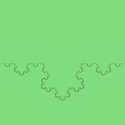
The first method is the idea that when a wave reflects off some complex geometry, one can 'low pass' the geometry based on the wavelength of the light, that is, one can ignore small bits of geometry below the light's wavelength as it has little effect. An approximation of this idea for simple fractals is to just look at the red and blue light frequencies, which are roughly different by a factor of 2, and use one more fractal iteration for the blue light than the red. The fractal I'm looking at is a simple 2D replacement of one directed line by two of equal length in a v shape:

If the two child lines are pointing along the same way then it produces a Levy curve, if both are flipped around then it produces a Koch curve, and if only one is flipped it produces a dragon curve. In each case the bend angle affects the dimension, which goes from 1D to 2D as the angle approaches 90 degrees. When I talk about the colour of such a 2D fractal, I mean when looking 'side on' to the curve, not from plan view.
Reflection Model
I model the surface as having no transparency, and reflecting light exactly. However I include a reflectivity. If the reflectivity is 100% then all the incoming light energy should be reflected back, regardless of the number of 'bounces', and regardless of the wavelength, therefore the curve is white. If the reflectivity is 0% then the curve is black. Firstly, I will look at the case where the reflectivity is very low but the diffuse sky intensity is very high, I therefore can approximate the colour by only looking at one reflection, and not multiple. It is expected that the colour will get paler as the reflectivity increases.
The first reflection model I call the diffuse model. Each vertex of the curve calculates the proportion of sky that is visible from its position, looking only to one side of the curve. It therefore models the reflection as going in all directions (as though from a point).


The second reflection model I call the reflect model, I model each vertex and the two line segments coming from it, as a (circularly) curved mirror. The light heading towards the camera therefore comes from a uniform distribution of directions which I calculate. The light level then represents the proportion of this angular section that is not occluded by the curve.
Levy Curve
For each model I show the fractal of dimension 1.2D, with colours as viewed orthogonally from above. Below that I show a map of the 1D view of the fractal as seen from above (horizontal) for increasing dimension 1 to 1.5 (vertical).
| diffuse model | reflect model |
|---|---|
  |
  |
  |
  |
The black areas in the top row are obstructions from the looping sections of the Levy curve, they have no colour as you are seeing the wrong side of the line (with flipped convexity too).
As you can see, the reflect model seems to give a bit stronger colour, but for both models the overall effect of the concave 'inside' of the Levy curve is a warm colour, and the convex 'outside' of the Levy curve is a colder colour, or much more neutral. It suggests concave is brown, convex is (slightly) blue. The result is also pretty much independent of the length of fractal used, or equally the chosen iteration count. It is also invariant to scaling the fractal by powers of two.
Koch curve
Because the Koch curve is built from subdivisions that flip direction each iteration, the shape difference at half the wavelength is is either concave or convex depending on the iteration, or equivalently the physical size of the curve. As such, and consistent with the results above, the Koch curve is either brown tinted when the difference is concave, or blue tinted when it is convex. Below I have shown the curve as viewed from above against dimension from 1 to 2 for both 9 (top) and 10 iterations, the double-resolution 10-iteration image is rescaled horizontally, so is the one with half height.
| Diffuse model | Reflect model |
|---|---|
 |
 |
 |
 |
Dragon Curve
This is the simplest case, looking the same on both sides and invariant to doubling the scale. Additionally, the overall colour varies little between the two models. Being 5% extra red at 1.2D and 10% at 1.4D. The lower images span dimension 1 to 2 vertically.
| Diffuse model | Reflect model |
|---|---|
  |
  |
Random Curve
Choosing a random bend direction between (-1,1) gives a colour that is slightly red on average, about 5% more red on both models, beyond about 1.4D.
| Diffuse model | Reflect model |
|---|---|
 |
 |
Conclusion
Both models are very coarse approximations of wave reflection off a fractal curve, but the similarity of results across two lighting models suggests the following results are quite general and probably valid:
- concave fractals are brown tinted
- convex fractals are only slightly blue tinted
- due to the asymmetry of above, random curves and dragon curves are slightly brown tinted
- Koch curves are brown or slightly blue tinted, flipping each scale factor of two, and flipping when you look from the other side
- these results are for the extreme case of a bright diffuse sky illuminating a curve with very low reflectance (so that we can ignore secondary reflections). Results will get paler, to white, as the reflectivity increases to 1.
- One can carry most of these results to 3D surfaces, though I imagine that a 1+k dimensional curve will equate closer to 2+√k dimensions in terms of colour.
Having said all of that, I have strong doubts about these conclusions. I have far more confidence in the following method of simulating light.
Coherent light
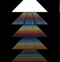
A perhaps more accurate simulation is to look at how a coherent directional light source reflects off the fractal, type 1 at the top of this post. Some work has been done on this by Jos Stam, his results indicate that the reflection goes from blue to white to yellow as the fractal roughness increases:

However, his work uses only a fractal height field, which isn't a proper fractal in that it doesn't have a simple fractal dimension. The high roughness results are unlikely to be accurate.
The approach I take is quite simple, I ignore secondary reflections (accurate if the absorption is high), from the view angle perspective, each point along the fractal that is not in shadow from the light incident angle will have a light travel distance l from light to point to eye. Each colour component (red, green, blue) is the magnitude of the sum of exp(ilf) where f is the frequency of that colour. This is simple interference; an approximation of the Kirchhoff integral.

above, the view angle and incident angle are -30 and 30 degrees respectively, and the curve is rotated to the view angle. The visible curve is that seen from the view angle and the black coloured part is in shadow. The light travel length for all the white points is used for the interference.
Unlike Jos Stam's work above, we cannot assume the integration is extended over the full curve as the curve varies everywhere. Instead we have to choose a finite width curve for the interference to act on. This finite size equates to the fact that our eyes can only resolve to a certain resolution (depending on the lens size), and features on the fractal under this 'coherence width' interfere. But this width is an extra parameter. The reflection off a Koch curve therefore has four pertinent parameters, which I map out in the image below. The first two (small coords below) are view angle (y) and incident angle (x). The third coordinate (the 8 rows) is the dimension of the curve, below it varies from 1 (top) to 1.2 (bottom). Notice that the top row is a line along view angle = -incident angle in other words pure reflection of the incoming light.
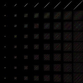
The fourth coordinate (the 8 columns) show different coherence widths from 6x red wavelength up to 48x red wavelength. In this paper the coherence width (as measured by the slit distance that causes the interfering waves to drop to 50%) is shown to go from about 7x sun's main wavelength in foggy/overcast sky to 80x on a clear day, so this corresponds quite well to the range I used.
There are clearly different colours in the reflected light, which would show themselves as glistening from a sharp light source. However, from a diffuse sky one must also integrate along any pixel row, and the overall colour on average is warm, with roughly 20% more red than blue.

Here we see an equivalent for a random curve. The profiles are a little less clear and asymmetric in the downward diagonal. But it remains the case that the average colour is similarly red-shifted.
Given the diagonal symmetry above for the Koch curve, we don't lose much by looking at just the downward diagonal (view angle = incident angle) and so we can plot the colour against just incident angle (small x) for continuously increasing dimension 1+n^2 for n=0 to 0.5, again each column is for increasing interference width:

Note that in this and the diagram above we only look at the few angles where the ray lengths on a flat surface cover an integer number of wavelengths, this prevents colour biases for these small coherence widths. This explains the small (and growing) width of each column.
As you can see, the reflections are colourful and show vertical lines that represent angles of high reflection where the angle increases with Koch dimension as expected. The lines have two properties, firstly they fade in an out, probably fading in when the continuous high reflection angle best matches the discrete displayed angles; secondly the line colour cycles through the spectrum with increasing fractal dimension, again as you would expect. Lastly the colours cycle more quickly with increasing dimension for the smaller wavelength light (columns to the right), which due to fractals' scale symmetry represents a wider coherent light wave, or more coherent light, and would give a more sensitive speckling.
The vertical lines just to the right of each column give the integration over all incident angles, so the colour of the curve if it were lit by light from all angles. It is less colourful but still varies between warm and cold, however, consistent with above, the average colour is red shifted.
The above images use very few view angles to avoid the colour bias, we can also avoid the colour bias by looking at the curve head-on, and can therefore look at a continuous increase in the colour frequency on the x axis, against increasing dimension downwards on the y axis:


Both images normalise the light wavelength relative to the 'lift height' of the curve for each dimension. The left image shows this directly and you can see the horizontal sinusoidal nature of the reflection intensity with light frequency, naturally this sinusoidal spectral intensity will be seen as a colour of hue that varies with the light frequency (relative to coherence width), on the right this is depicted... one can think of the x axis as now representing an increase in the coherence width (more coherent light).
We can also choose to ignore the colour bias from view angle and just display the continuous view angle (x axis) against increasing light frequency (downwards) for five dimensions from roughly 1 to 2.
Notice that as the dimension increases it tends towards two vertical bars (the separation or view angle difference, increasing with dimension). These bars represent the increasingly flat (high reflectance) sides of the Koch curve that becomes a triangle at dimension 2. Intermediate dimensions show speckled patterns that cause both glimmering and colours. Interestingly these appear quite fractal-like in themselves, probably a polar plot would be less distorted.
All the above were for a single Koch curve patch over the coherence width, which in reality is usually very small. It remains to consider what the macroscopic fractal will look like. We must apply the same interference for all pixels along the width of the macroscopic fractal:
Since we can't limit to integer view angles, we choose a different means to avoid colour biasing due to the finite coherent width (which we make about 2 pixel widths), firstly we weight the light contributions to ramp down at both sides of the light beam (a parabola, see bottom of figure below), secondly we make the higher wavelength light have a proportionally higher coherence width, as shown in the figure below.

Below we show such a fractal lit directly head on (left) and lit one radian from the left side (right). for increasing coherence width (downwards) from 1 pixel to 8 pixels. Each column is increasing dimension from 1 (top).


The result is that the coherence width makes almost no difference to the colour of the fractal. As expected the fractal is more blurry with a larger width and for very small width (hardly any coherence) the colour tends to white. Average colours are shown down the right hand line, and you can see they are very consistent. One can also see that the fractal colour changes greatly with dimension, and varies a little across the length of the fractal.

Above is the average over 20 light angles, so for an ambient white sky. The colour is much less pronounced however you can still see a definite change in the hue with increasing dimension, and the colour strength increases with higher dimension, though the fractal also becomes darker.
Given that the coherence width makes little difference, what if we use a fixed width (say 2 pixels) and increased the scale of the fractal? here's what happens for a point light source, head on (left) and 1 radian from the left side (right):


In both cases we see a hue cycling with curve scale (y axis) and an increase in the cycle density with increasing dimension (lower rows). This matches the result from the first section of this post, where blue vs red tinted Koch curves toggle as the iteration order increments (equivalent to increasing size). The above is just more realistic as it has a more correct frequency ratio between blue and red light (rather than 2) and it includes green light properly.

The ambient white sky (above) also shows this hue cycling, but the colour is more grey, particularly for low dimension curves.
We can also copy this method for the other fractals:
Levy convex (left) and concave (right):


Dragon (left) and random (right):


Here's a spinning Koch snowflake which combines ambient light with a point light source from the right hand side:

and here it is without the point light, so just directional light. Notice that the vertical spectrum flips every 30 degrees, so browns become purple/blue and visa versa. This exactly matches the observation in methods 1 and 2 in the first section of such a flip when viewing the curve from inside compared to outside. This is because a 30 degree turn is equivalent to seeing the curve from the opposite direction. This is a very interesting property of the Koch curve.

and finally, here's another attempt with a wider spot size for a large scale Koch snowflake with a stronger point light, it shows the much more dramatic colouring you get from coherent light sources:

By comparison, here are the gifs for the levy curve and dragon curve respectively, just ambient and lit, click for larger versions:


dragon curve:


Conclusions for Coherence Approach
- The first three diagrams seem to confirm the previous general conclusion that a red-shift seems to be the average shift for a Koch curve as well as a random curve.
- The idea that the Koch curve hue cycles with its scale is consistent in all the above examples.
- colour is more prominent as the fractal dimension increases
- colour is more prominent on single point light sources, and less on more spread out light sources.
- In all cases, the hue varies more with curve scale (where it fully cycles) and with increasing dimension, and less so along the length of the Koch curve.
- The last figure shows that colours are stronger in the hollows... this is because the incident light angle range is less, so it is closer to the point light source case. This is consistent with the first section where the concave Levy curve shows stronger colour than the convex one.
Overall Conclusion
The three versions of light dynamics suggest the following strongly:
- coloration increases with curve dimension but brightness decreases
- coloration increases (but brightness decreases) with decreasing reflectivity
- most fractals of moderate dimension will be quite dark compared to smooth surfaces, so coloration is most likely visible under strong light
- coloration increases with more pointlike light sources, but is still noticeable for ambient white light. Therefore coloration is stronger in concave areas.
- coloration is not really effected by coherence width (how wide the area where interference occurs), only reduces for very small width.
- hue cycles with scale of the Koch curve (first sections suggest it doesn't really do this for Levy curves)
The code for the latter images is available at: https://github.com/TGlad/FractalColour2D
A more concise summary is given here: https://sites.google.com/site/tomloweprojects/scale-symmetry/what-colour-are-fractals.
I'll finish with some more well known fractal curves, now in colour:
Minkowski sausage:


Minkowski mushroom: (I made up the name):


Vicsek fractal:


If you would be willing to share more regarding your Fractal Automata and Fractal Reaction-Diffusion algorithms, such as in a code or algorithm exchange and collaboration, please let me know. I am happy to share my source, as Jason Rampe a.k.a Softology and I have done which rendered excellent results.
ReplyDeleteI believe there is overlap in those two algorithms of yours and some of mine, which might result in new and novel algorithmic derivatives for us both.
A subset of the algorithms which a collaborative relationship would grant you may be seen at the following link, though this is a tiny fraction of the whole.
https://www.flickr.com/photos/gds-entropy/
Do consider the offer, and please let me know your choice; little time, interaction or effort is required and the benefits are both mutual and potentially significant.
I may be reached at [mail split to avoid spam, symbols rendered as words]:
gds
hyphen
entropy
at
Hotmail
dot
com