There is an interesting extension to bidirectional Laplacian growth, which should generate 'wide' tree structures (a tree-tree to use my terminology).
The idea is to have two sources of chemical (A and B) which both diffuse with equal diffusion rate from their sources (in our example, a line at the top for A and a line at the bottom for B). There is then a single scalar field C that is both grown and shrunk by interacting with these A and B chemicals (in our example the boundary starts midway between the two lines). A and B are both set to 0 at the boundary of C, so the growth is based on the gradient at the boundary dA and dB, using the formula:
growth rate of C = g((dA^a)(dB^b)-s)(dA - dB).
Note that the growth rate of C is signed, so the boundary can grow or reduce.
The g value just dictates the rate of growth. For good results it should be slower than the diffusion of A and B, if it isn't then you can get dynamic behaviour with pulsating growths.
The s value represents smoothness, when it is smaller then thinner trees are accepted.
The a and b values represent the relative important of the two chemicals in building the tree. When a is small the branches filled by chemical A are thinner, and vice versa.
Implementation
As seen in the previous post, there are multiple ways to implement this idea:1. Using a shader, run the diffusion, and allow a slight gradient to C, with some careful interaction to achieve the formula above. Conceptually simple, but slow (particularly in 3D).
2. Use the fuse-breakdown paper as a model to grow it stochastically on a grid (but without the diffusion component or the random walk).
3. Model the boundary as a polyline with one 1/x drop off per vertex, using the fuse-breakdown model, but not stochastic, growth the whole line.
4. Alternates: we might do a combination of 2,3, or a hybrid of 1,3 like the coral paper, basically a shader for the diffusion and a curve for the growth.
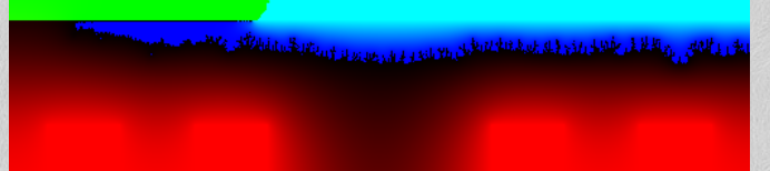
I have used method 1, and preliminary results are as follows:
Chemical A is diffused from the bottom as 5 red sources (to give a variation). Chemical B is the cyan bar on top. a=b=0.5, s=0.0025

If we remove the middle red source then the bounary drops down in the middle, and gets smoother. That is a consequence of the method, the boundary is smoother where the chemical concentrations are less:


Update:
Using proper gradients (not just neighbour pixel values)
Here are progressively smoother versions from s=0.05 up to s=0.8 (a,b=0.5):
Here are progressively smoother versions from s=0.05 up to s=0.8 (a,b=0.5):


The power of a,b seems to change it from super-fractal (rough at small scales) to sub-fractal (smooth at small scales), from 0.125 to 2:


We can also define a power on the difference, i.e. g((dA^a)(dB^b)-s)(dA^n - dB^n). We might expect larger n to be more directed as it is with DBM, here it is from n=0.5 to n=2:


As you can see, there is not a lot of difference in the results here. This could be that the actual gradients are too approximate to yield a strong difference. But we can see something... the boundary starts as a slightly sine wave, and the n=0.5 has held and exaggerated that broad wave more then n=2. This seems more the opposite of what I'd expect.
The current algorithm (s=0.2,a,b=0.5,n=1) does grow towards targets... but seemingly only slightly:

A consequence of the model is that the growth is faster and more erratic closer to the source, and really starts to move like something on fire, as the growth balances with the diffusion of the chemicals (like air and the combustible compound).
Here's another asymmetrical one (a=0.45,b=0.55), notice the branching is more upwards:

It currently suffers from the upwards branches coming and going in repeated manner, and not as much height variation as for equal a,b for some reason.
Here's another asymmetrical one (a=0.45,b=0.55), notice the branching is more upwards:

Update
Here I have made one source the centre and another source the surrounds:

This is a little different, I have made the initial sources self-perpetuate by scaling up the chemicals everywhere by a small amount, to counter the boundary which is a sink for both chemicals. The consequence is that the blob doesn't have to remain around a spherical source. But if the scaling is too great, then large branches can literally bud off into new blobs.
Instead of grown the shape pixel by pixel stochastically, we can grow it using the value of the boundary channel to give sub-pixel accuracy. The result is quite similar:

One difference is that the stochastic one doesn't symmetry-break as easily, so it takes longer for smooth surfaces to become rough. On the other hand, in cases where the result should be smooth, it models the smoothness better. Using stochastic or not is just a boolean flag. Since this version isn't stochastic, it is symmetric if the original circle boundary (and chemical distribution) is exactly symmetric:

The pattern here is just a function of the imperfect disk rendered to pixels.
No comments:
Post a Comment