Saturated and desaturated shapes

Here's an unusual curve:

Its fractal dimension is 1, so it is not a fractal. But its length is infinite. It is constructed like a Koch/Cesaro curve with local dimension D(i) at iteration i given by D(i) = 1+1/i. Where the per-iteration bend angle equals 2asin(exp(-ln(2)/D(i))).

The question is how do you compare the lengths of different subsections of the curve, if they're all infinite? This is reminiscent of the Coastline paradox. 

There are related curves that have local dimension D(i)=1+0.5/i and 1+2/i respectively:

This raises a second question, not only do we not know which is longer, but they clearly change in how lumpy they are. How do we measure that? 

I described them all as lumpy, rather than 'rough' like fractals because the lumps are only at the larger scales. I use the term saturated to describe these curves. Their length has saturated to infinity and it also invokes the idea of a shape saturated and swollen with water like wrinkly fingers in the bath.

This next curve has local dimension D(i) = 1.2618+1/i so it is a fractal, in fact it is the saturated version of the Koch curve. Its fractal length (fractal content or Hausdorff measure) is infinity.

Moreoever if you measured this fractal content for a slightly higher dimension such as 1.2619, it would be zero. So you cannot use fractal content to measure the length of this curve either.

The answer to these problems is that instead of measuring these lengths in metres (or metres^1.2618 for the saturated Koch curve) you measure the in m log^n m (or m^1.2618 log^n m respectively). In general any shape of dimension d that is saturated can be measured in m^d log^n m. Here n is the value that describes their lumpiness. In these examples when the local dimension is D(i) = D + k/i, then n = k ln(2).

The shapes don't have to be curves. This is a particularly pure case of a saturated 0D shape, i.e. a point or finite number of points, where D(i) = 0 + 1/i:

There are infinite points in this saturated shape, but unlike the 2D Cantor set its fractal dimension is still zero, so it is not a fractal. But, you can still compare the size of these shapes (or portions of them) as they can be measured in log^n metres. Here is a twice as saturated set of points (twice n): D(i) = 0 + 2/i:

The point spacing is decreasing as we zoom in. Indeed all of the above examples change their scale and shape as you zoom in. But even though their log-log plots are curved it is still possible for shapes to be scale-symmetric. Take for instance these binary trees:

They both have fractal dimension 1 so are not fractals, just connected lines. If the stem length is 1m then the left image has total length 12 m. But the right shape has infinite length; it is saturated. We can still measure its "length" as 2.88 m log m. This saturated tree occurs when the child branch lengths are exactly half the parent branch length. 

Desaturated shapes

The same thing happens in the other direction. You can take a 2D area and remove the harmonic series. Here the local dimension is D(i) = 2 - 1/i, and 2 - 2/i respectively. They both have area zero, so how do we compare their sizes?

Similarly you can also desaturate a fractal, such as the Koch curve here, using D(i) = 1.2618 - 1/i. Its fractal content is then zero.

The equivalent measurement for these is to measure in m^d / log^n m.

Here's a desaturated solid triangle, with D(i) = 2 - 1/i:

I call these desaturated as their d-volume has all of its size "dried" out of it, like dried ground that has split. In general we can think of these desaturated shapes as dessicated or depleted versions of the original shape.

This next shape is a line using a binary subdivision formula with D(i) = 1 - 1/i:

It looks like a Cantor set but its fractal dimension is 1 and its 1D length is 0. You must measure the size of this desaturated line in m/log^n m.

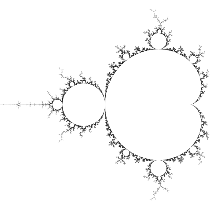
These aren't the only shapes that act this way. If we plot the box counting dimension of the boundary of the Mandelbrot set as a log-log graph, then we plot the function y=-2(x-s) - g log_2(-(x-s)), we see that it fits quite well to the curve when s=18.6, g=3.8:

This function when translated to a gradient error with its fractal dimension of 2, is also a 1/x harmonic function. The close match is suggestive (but certainly not proven) that the Mandelbrot set's boundary is also a desaturated area, with n equal to g. This would explain some previous suggestions that the boundary's area may be zero despite it having dimension 2.

Above: compare the outer Mandelbrot boundary with the next largest minibrot to see how much denser the boundary gets as you zoom in. (image thanks to Claude). 

If the above function is close then you can convert it to the physical quantity formula by replacing x with ln(1/x) and taking 2 to the power of y. The resulting formula tends to m^2 / log^n m for large x, giving the size of the Mandelbrot set boundary as: 3026 m^2 / log^3.8 m.

But we don't know that the function needs to reach down to the 1 box level (y=0), the function only needs to be asymptotically correct (for large negative x). 

It also isn't necessary to have the same s in both parts of the formula, so with different values we can get more curvature in out best-fit curve by dropping n to 2, when s1 = 14.3 and s2 = 12.7 we get a size of:

15 m^2 / log^2 m:

If n = 1 then s1 = 12.3 and s2=9 is a good fit, so you get a size of: 1.36 m^2 / log m:

Both of these seem somehow more likely than n=3.8. But we would need more data to make a better guess on n, which describes how desaturated (dessicated) the boundary is as a 2D region. 

The function to simplify in these cases is: y=2^( -2(log(2,k/x)-s1) - g*log(2, s2-log(2,k/x))), where k is the number of pixels per unit in the image, which is 3600 for this case.